Advanced Topics

Integrating Snowflake into Planful using the new Snowflake Native Connector

Overview: Data Flow from Snowflake to Planful

Data Flow Summary: A native Snowflake connector in Planful allows you to pull General Ledger (GL) / Segment hierarchies/ External Source model data directly from your Snowflake data warehouse into Planful’s planning platform. Planful acts as a client to Snowflake, executing SQL queries on your Snowflake instance and importing the results into Planful’s data model. This integration ensures that your financial models in Planful are fed with up-to-date GL data from Snowflake without the need for manual CSV exports or complex ETL processes.

Note:

This Native Connector functionality is available as a Opt-in. Contact your Account Manager to enable the Snowflake Integration feature.

Flag Name: Is_Snowflake_Enabled

How the Integration Works: Once the connection is set up, Planful uses Snowflake’s APIs/drivers to query the GL data:

• Planful (as a SaaS tool) initiates a secure connection to Snowflake using provided credentials or keys.

• Planful sends a SQL query (either a default query or one you configure) to Snowflake to retrieve the desired GL records (e.g. journal entries, account balances).

• Snowflake executes the query in a specified warehouse and returns the result set over the encrypted connection.

• Planful then imports that result into its application.

This direct pipeline means any updates in Snowflake (e.g. new journal entries or adjustments) can flow into Planful on the next refresh. The diagram below illustrates the high-level flow:

Connection Setup Insights & Recommendations

Setting up the connection involves configurations on both Snowflake and Planful. On the Snowflake side, you’ll prepare a user/role with proper access and (if necessary) adjust network settings. On the Planful side, you’ll configure the Snowflake connector with the appropriate credentials and connection details.

Snowflake Configuration (Roles, Permissions, Networking)

1. Create a Read-Only Role for Planful: In Snowflake, create a dedicated role (e.g. PLANFUL_READ_ROLE) with read-only access to the relevant GL tables or views. Grant this role usage on the database and warehouse, and SELECT on the specific schema or tables that contain GL data. For example, you might run SQL commands like:
   

   CREATE ROLE PLANFUL_READ_ROLE;
   GRANT USAGE ON WAREHOUSE finance_wh TO ROLE PLANFUL_READ_ROLE;
   GRANT USAGE ON DATABASE finance_db TO ROLE PLANFUL_READ_ROLE;
   GRANT USAGE ON SCHEMA finance_db.gl_schema TO ROLE PLANFUL_READ_ROLE;
   GRANT SELECT ON ALL TABLES IN SCHEMA finance_db.gl_schema TO ROLE PLANFUL_READ_ROLE;
   -- (Adjust scope to grant only what's needed, e.g. specific tables instead of ALL TABLES)

   These grants ensure the role can read the GL data but not make any modifications. Following the principle of least privilege, limit this role’s access only to the data Planful needs (e.g., the general ledger fact table and perhaps related dimension tables). This minimizes security risk while allowing Planful to retrieve data.

2. Create a Snowflake User for Planful: Next, create a new Snowflake user account (service account) that Planful will use for the connection. For example:

   CREATE USER Planful_user
   PASSWORD = '<<strong-password>>'
   DEFAULT_ROLE = PLANFUL_READ_ROLE
   DEFAULT_WAREHOUSE = finance_wh
   MUST_CHANGE_PASSWORD = FALSE;
   
   GRANT ROLE PLANFUL_READ_ROLE TO USER Planful_user;

   Choose a strong password if using username/password auth, or prepare to use key-pair auth (discussed below - And it is most recommended). By assigning the read-only role to this user, you ensure that any queries Planful runs will execute under that role’s privileges. We recommend setting the user’s default warehouse to the one you want Planful to use (e.g., a warehouse sized appropriately for the data volume), so that Planful’s queries always run there. Ensure the warehouse has auto-suspend enabled to avoid incurring costs when not in use (this way, Snowflake will automatically start the warehouse when Planful queries and shut it down after idle time).

3. (If Applicable) Whitelist Planful’s IP Address: If your Snowflake account has a Network Policy restricting inbound connections by IP (for example, if Snowflake is configured to only allow known corporate IP ranges), you will need to add Planful’s servers to the allowlist. Planful is a cloud service, so obtain the outbound IP address(es) it uses for Snowflake connections (Planful’s documentation or support can provide these). Then update your Snowflake network policy, for example:

   ALTER NETWORK POLICY my_policy
   ADD ALLOWED_IP_LIST = ('<Planful_IP_Address>');

   (If you don’t have a network policy in Snowflake, by default Snowflake accepts connections from any IP, so this step is only needed in restricted environments.) Note: Snowflake’s network policies can include lists of allowed IPs or ranges. Make sure to include all IP ranges Planful might use. If Planful’s IP changes or if it provides a range, update the policy accordingly. Skipping this step in a locked-down Snowflake will result in connection errors until the IP is allowed (you might see errors indicating Snowflake cannot be reached, SqlState 08006, etc., which signal network blocks).

4. Test Snowflake Setup: As a sanity check, you can test connecting to Snowflake with the new user. For instance, use Snowflake’s web UI or SnowSQL CLI to log in as Planful_user (with the password or key) and verify you can SELECT from the GL tables and nothing more. This ensures the permissions are correct before configuring Planful.

Once Snowflake is ready, configure the connection in Planful:

1. Locate the Snowflake Connector in Planful: In Planful’s interface, navigate to the Integrations or Data Connections section (often from your workspace homepage). Choose to add a new connection, and select Snowflake (Planful’s native Snowflake integration). Planful will prompt you for Snowflake connection details.

2. Enter Snowflake Connection Details: You’ll typically need to provide:

   • Account Identifier: This is your Snowflake account URL or ID. For example, Planful might ask for the Snowflake account in the form orgName-xyz12345.snowflakecomputing.com or the shorter account ID and region (check Planful documentation for the exact format they expect).

   • Warehouse: The name of the Snowflake warehouse to use for queries (e.g., FINANCE_WH). This should match the warehouse you granted usage to the role. Planful will use this warehouse to execute the GL queries.

   • Database and Schema: The default database and schema where your GL data resides (e.g., FINANCE_DB and GL_SCHEMA). This helps Planful know where to run the queries. (You can usually change schema in your SQL, but providing defaults is convenient.)

     • Role: You can create the read-only role (PLANFUL_READ_ROLE) and ensure the user’s default role is correctly mapped to this role.

   • Credentials / Authentication: Provide the authentication method and credentials. This could be:

     • Username & Password: Enter the Snowflake user (Planful_user) and its password. (Ensure you store the password securely and rotate it periodically.)

     • Key-Pair Authentication: Planful supports Snowflake key-pair auth, which is often recommended for cloud integrations. In this case, you will upload or paste the private key associated with the Snowflake user (and possibly a passphrase if the key is encrypted). Planful will use this key to authenticate instead of a password. (See the Authentication section below for details.)

3. Test and Save the Connection: Planful recommends testing the connection. Ensure Planful can successfully connect to Snowflake. If the test passes, save the connection. If it fails, re-check the details:

   • Typos in account names or credentials are common issues.

   • If you see a network or timeout error, double-check the IP allowlisting (if a network policy is in place) to be sure Planful’s IP is allowed.

   • If you see a Snowflake permissions error, verify the user has the right role and grants (e.g., SELECT privilege on the target tables).

4. Configure the Data Import Query: After the connection itself is set up, you will specify what data to bring in. Planful may allow you to write a custom SQL query or simply select a table to import. For GL data, you might write a query like: SELECT FROM FINANCE_DB.GL_SCHEMA.GL_TRANSACTIONS WHERE DATE >= '2024-12-01'; or join with dimension tables if needed. (See *SQL Scripts** below for examples.) Input your query or table selection in Planful’s import configuration at the DLR level.

5. Run an Initial Import: Execute the import job in Planful to pull data now. This initial run will populate Planful’s data model with the Snowflake GL data. Confirm that the data looks correct in Planful (row counts, sample values) to validate the entire pipeline.

By completing these steps, you’ve established a live connection from Snowflake to Planful. The Snowflake side handles authentication and data serving, while Planful periodically uses this connection to fetch the latest GL records.

Tip

Document the connection setup (Snowflake user name, role, what tables are included, etc.) for future reference. This will help when team members need to know how data is flowing or if you need to troubleshoot or update permissions later on.

Access Controls and Security Recommendations

In summary, the Snowflake–Planful integration transmits data securely (TLS-protected), and Snowflake ensures the data is encrypted on its side. You should avoid non-secure channels (e.g., don’t export GL data to an unencrypted CSV/email when a direct connector is available). Using the native connector means you inherit Snowflake’s robust security for data transfer.

Role-Based Access Control (RBAC) and Network Restrictions

• Snowflake RBAC: Snowflake uses a role-based access control model to restrict what each user or integration can do. So, it is recommended to create a limited role such as PLANFUL_READ_ROLE. In general:

  • Privileges (like SELECT on a table) are granted to roles, and roles are then assigned to users. In our case, the PLANFUL_READ_ROLE has SELECT on the GL tables, and the Planful_user is assigned that role. This means Planful (using Planful_user) can only read those tables and nothing else (it cannot, say, delete data or read other schemas). This protects your data by sandboxing the integration.

  • Least Privilege Principle: Always ensure the Snowflake role used by external tools has the minimum permissions necessary. For example, if Planful only needs GL data, don’t grant it access to HR or sales data. This limits exposure if the credentials were misused and also prevents accidental access to unrelated data.

  • Object Access Management: You might manage more complex scenarios by using Snowflake views or secure views to expose exactly the data needed. Some organizations create a dedicated schema with curated views (e.g., a view that already filters out confidential fields) and give the Planful role access only to those views. This way, even within the GL table, you control columns and rows Planful sees. Such techniques can complement RBAC.

• Network Policies: Snowflake network policies are another layer of defense. As noted, by default Snowflake allows connections from any IP, but admins can restrict access to specific IP ranges. If your company has enabled this, you must include Planful’s outbound IP addresses in the allowed list for the Planful connection to succeed. In practical terms:

  • Work with Planful Support (*Planful Ops/security team will provide this detail as applicable for the hosting environment like AU01/NA01 etc.*,) to get the list of Planful’s IP addresses. These are the IPs from which Planful’s servers will connect to Snowflake.

  • Add those to Snowflake via a network policy (or update an existing policy). Snowflake network policies can be set at the account or user level. You might choose to apply it at the user level for Planful_user only (thus only that user is restricted to Planful’s IPs), or at the account level (all users – if applicable). User-level network policy could be ideal here: it means even if someone somehow got the Planful_user credentials, they couldn’t connect from an unauthorized network location.

  • This IP dependency must be well-documented to prevent downtime when IP ranges change or tenants move across different Planful environments. Work with Planful to obtain and maintain updated IP ranges whenever changes occur.

• Other Security Best Practices:

  • Monitoring and Auditing: Snowflake provides a query history and login history – you can monitor that the Planful_user only runs expected queries at specified intervals only.

  • Secrets Management: Treat the Snowflake credentials or keys you put into Planful as secrets. Only share them on a need-to-know basis. Planful will encrypt these and store at Planful side.

  • Planful Permissions: Within Planful, manage who can edit or trigger the Snowflake data connection via Cloud Scheduler Process Flow and the DLRs. You wouldn’t want an unauthorized Planful user to be able to alter the Snowflake query or credentials. Use Planful’s  navigation and access controls to restrict access to integration settings.

SQL Scripts to Retrieve Data - Recommendations and Strategies

With the connection in place, the next step is to write SQL queries that fetch the General Ledger data you need. As a business analyst, you might not need to write very complex SQL if the data is clean, but understanding the basics will help you get exactly the slice of data required. Below we outline example queries and how to manage them:

Basic SELECT Queries: Planful’s Snowflake connector allows you to specify a query (or sometimes simply select a table). Often, you’ll start with a SELECT statement to pull the GL records. For example:

• Retrieve all GL entries for a certain period: If you want the general ledger transactions for fiscal year 2024, you might query by date:

SELECT
    transaction_id,
    account,
    department,
    amount,
    posting_date
FROM finance_db.gl_schema.gl_transactions
WHERE posting_date >= '2024-01-01' AND posting_date < '2025-01-01';

This will select columns like transaction ID, account, department, amount, and date from a gl_transactions table, filtering the rows to only include those in 2024. In Planful, you could use a parameter for date/month/year when the tool supports it, or edit the query as needed for different time frames via DLR Query editor!  

Filter by department or other dimensions: Perhaps you only want ledger entries for the Sales department or a specific business unit. You can add conditions:

SELECT account, posting_date, amount
FROM finance_db.gl_schema.gl_transactions
WHERE department = 'Sales'
AND posting_date >= '2024-01-01' AND posting_date < '2025-01-01';

This would feed Planful only the Sales department’s ledger lines for the year. Filtering at the SQL level is important for performance – it’s much more efficient to let Snowflake return only needed rows than to fetch everything. Snowflake is optimized for these set-based filters.

Aggregating or pre-calculating (if needed): You can have SQL do data aggregations. For instance, to retrieve monthly totals per account you could query:

SELECT
    account,
    DATE_TRUNC('month', posting_date) AS month,
    SUM(amount) AS total_amount
FROM finance_db.gl_schema.gl_transactions
WHERE posting_date >= '2024-01-01' AND posting_date < '2025-01-01'
GROUP BY account, DATE_TRUNC('month', posting_date);

This returns one row per account per month with the summed amount. Planful could then import this summary. Decide based on your use case – Planful can ingest detailed data or aggregated data depending on what your model needs.

Managing and Validating SQL Queries:

• Testing Queries: It’s best to test your SQL outside Planful first. Use Snowflake’s worksheet/web UI or any SQL editor to run the query and inspect results. Verify that the data returned looks correct (e.g., correct date range, no duplicates, expected number of records). This helps catch issues early (like a filter that’s excluding too much or not enough).

• Performance Considerations: GL tables can be large (millions of rows). Use filters (WHERE clauses) to limit data whenever possible. Also select only the columns you truly need (for example, if Planful only needs amount and account, no need to select every column). This reduces the data volume, speeding up the transfer. Snowflake’s warehouses can handle big queries, but unnecessary large result sets will slow down the import.

• Use of Views or Stored Logic: If your GL data requires joins or calculations (for instance, joining account codes to descriptions, or converting currencies), you have a couple of options.

  • One convenient approach is to create a materialized view in Snowflake that encapsulates this logic. For example, a view v_gl_transactions_filtered might join the chart of accounts and filter out certain system entries. You can then **SELECT FROM v_gl_transactions_filtered* in Planful.

    • The benefit is twofold:

      1. Snowflake can optimize the view’s query, and

      2. if you need to change the logic, you can update the view in Snowflake (which is often version-controlled via SQL scripts or a tool like dbt) rather than modifying the query in the Planful UI. This provides better change management for complex logic.

• Version Control and Documentation: Treat the SQL query powering your Planful import as a piece of source code for your data pipeline.

  • Document what each query does (e.g., “This query pulls the last 2 months of GL transactions excluding inter-company entries”). This helps future maintainers and auditors understand the data lineage.

• Validation: After Planful imports the data, do a quick reconciliation against Snowflake. For instance, if you imported a sum of amounts by month, cross-check that the total matches between Planful and a Snowflake query. This ensures the data was transferred correctly and completely.

SQL Query Management in Planful: Planful provides an interface to input the SQL and perhaps a preview of data at the DLR level. When saving the import configuration, Planful may validate the SQL (checking syntax or trying a small preview). If there’s an error (syntax error, or a privilege issue), Planful will display it. Common mistakes include missing a semicolon (if required) or not fully qualifying table names (it’s best to use database.schema.table in cross-database queries since Planful’s session might not have a context set, unless you set the default database/schema in the connection).

In summary, writing SQL for GL data is about selecting the necessary data and filtering out the rest. Keep queries as simple as possible, test them thoroughly, and leverage Snowflake’s power (through views or aggregations) to lighten the load on Planful. By managing these queries carefully and possibly version-controlling them, you ensure that the data import process is reliable and transparent.

Data Loading - Scheduling & monitoring recommendations

Once the connection and query are configured, you’ll want to automate the data refresh so Planful stays in sync with Snowflake. Here’s how data loading and scheduling typically works, along with error-handling and monitoring best practices:

• Scheduled Refreshes: Planful allows you to schedule imports on a regular cadence. For example, you might schedule the GL data import to run nightly at 2 AM or every hour. The frequency depends on your needs (for financial data, daily refresh might be sufficient, or intra-day if you need more up-to-date numbers. To schedule, use Planful’s Cloud Scheduler Process flow interface. Once set, Planful will automatically execute the Snowflake query at those times and update the dataset in Planful.

• On-Demand or Triggered Refresh: In addition to fixed schedules, you can usually trigger a refresh manually (e.g., press a “Refresh now” button if you made an urgent update in Snowflake and need it immediately in Planful). Some advanced setups allow event-driven updates – for instance, using Planful’s API to trigger a Process Flow.

• Incremental vs Full Loads: If the volume is large and growing, consider using a date filter like “WHERE date >= last 30 days” for frequent refresh, or have Planful only pull changed data. This is an optimization to discuss if needed – initially, a full refresh might be simplest and then you can optimize for Performance.

• Error Handling: It’s important to handle errors gracefully:

  • If the Snowflake query fails (due to syntax error, or maybe Snowflake being unavailable), Planful should report the error. Typically, you’d see a message in Planful’s import log such as Data Load History or detail Process flow log for exceptions or errors. Monitoring these logs is crucial. Good to set up an alert via new Sumo log based Customer Command Center views for proactive monitoring.

  • Planful will send notifications on import failures so these can be monitored!

  • Common error scenarios: network issues (Planful can’t reach Snowflake – check network policy or Snowflake outage), permission issues (someone altered the Snowflake role’s grants – the query will suddenly fail to select from a table), or table may not exists or data issues (the query itself runs but returns unexpected results, e.g., nulls due to upstream changes) ! .

  • Have a procedure for errors: for instance, if a refresh fails, Planful keeps the last good data. You need to, investigate the error in Planful logs and Snowflake’s query history. Snowflake’s QUERY_HISTORY view can show if the query was executed and if it threw an error.

• Monitoring & Best Practices: Proactively monitoring the data pipeline ensures reliability:

  • Regular Audits: Verify that the data in Planful matches Snowflake’s source. For example, run a monthly check on the GL totals in Planful reports equal those in Snowflake or your source system. This catches any discrepancies possibly caused by missed updates or integration issues at appropriate granularity.

  • Performance Monitoring: Check how long the Snowflake query takes and how long the Planful import takes. If a refresh is running slow (or nearing your schedule interval so they start overlapping), consider optimizing the query or increasing the warehouse size temporarily. Snowflake’s UI or Account Usage views can show you query run times and resource consumption.

  • Warehouse Management: As noted, set the warehouse to auto-suspend and auto-resume. Planful will trigger auto-resume when it connects. If the data volume is large, ensure the warehouse is sized adequately to handle the query quickly (you can use a medium/large warehouse for the minute it runs, which might be more cost-effective than a small warehouse running for a long time).

• Concurrent Load Considerations: If you have multiple imports (GL, budgets, other data) hitting Snowflake at similar times, be mindful of warehouse load or Snowflake credit usage. You might schedule them staggered or use separate warehouses if needed to balance load.

In practice, once scheduling is set up, the process is mostly hands-off. Monitor it and address issues when they arise. Leverage Planful Cloud Scheduler→ Job Manager, or Data load history to track the load status within Planful.

By following these practices, you’ll ensure that Planful always has timely GL data and that any hiccups in the pipeline are quickly identified and resolved, with minimal impact on the business users relying on the data.

Dynamic Planning: Model Sizing Insights

Introduction

In model sizing, the three main factors—Key, Value, and Record count—work together to determine the overall capacity and physical storage of your model. Here’s how they interact:

1. Key Dimensions:

   • The Key Member Count is calculated by multiplying the number of members in each Key dimension. This product represents the maximum theoretical number of unique key combinations (or potential data blocks) that your model can support.

   • For example, if your Key dimensions are Account=80, Company=10, Department=60, Product=30, and Project=40, then the maximum theoretical keys would be 80 × 10 × 60 × 30 × 40 = 57,600,000.

2. Value Dimensions:

   • The Value Member Count is similarly calculated by multiplying the number of members in each Value dimension. This tells you the maximum number of tuples (cells) that a single data block (or “value block”) can theoretically hold.

   • For instance, if your Value dimensions are Scenario=3, Location=15, and Measures=2, then each data block can hold 3 × 15 × 2 = 90 tuples.

3. Record (Data Block) Count:

   • In practice, not every possible key combination is populated. Instead of storing each tuple individually, Database stores a data block for each key combination that actually has data.

   • The Records column (visible under Manage > Application Statistics) shows the actual number of these populated data blocks.

4. Physical Storage Size:

   • Each data block has an associated storage size (reported in MB), which is influenced by the number of tuples in the block and the Database’s compression.

   • The total storage size is the sum of the sizes of all these data blocks.

Insights:

• The theoretical capacity of your model is defined by the product of Key and Value dimensions, but the actual storage depends on which key combinations are used (i.e. the Record count).

• A high Key Member Count with a low Record count indicates that many potential combinations are empty.

• The Value Member Count sets an upper limit on how much data a single record can hold; if a record is only partially populated, its physical size is smaller.

• Overall, when assessing model sizing, you want a balance: your Key/Value structure should support your reporting and aggregation needs without unnecessarily increasing the number of populated records and, consequently, the on-disk storage size.

Practical Explanation of Application Statistics

Below is an explanation of how Key Member Count, Value Member Count, and Records come together to influence model sizing in the context of your data. The core ideas remain consistent across all the models, but we’ll highlight a few illustrative examples to show how these numbers interact.

1. Key vs. Value Dimensions

• Key Dimensions define the unique “key combinations” for your model.

  • Multiplying the member counts for all Key dimensions gives the maximum theoretical Key Member Count.

  • Each unique key combination (if populated) will become a record (a data block) in the database.

• Value Dimensions represent additional “value slots” for each key combination.

  • Multiplying the member counts for all Value dimensions yields the Value Member Count, i.e., the maximum number of tuples/cells that can be stored in each data block.

• Records (Data Blocks) are only created when a key combination actually has data. Hence, Records ≤ Key Member Count in practice.

2. Interpreting the Columns

1. Key Member Count:

   The theoretical maximum number of key combinations (data blocks) the model can hold.

2. Value Member Count:

   The maximum number of “slots” or tuples per data block.

3. Records:

   The actual number of data blocks that currently store data (often far less than the theoretical Key Member Count).

4. Size (MB):

   The total compressed size on disk for all data blocks in that model. Even if the Key Member Count is huge, the size might be small if only a subset of records is populated—or if data compresses well.

3. Example Models

4. Key Insights on Sizing

1. High Key Member Count ≠ Large On-Disk Size

   • Even if you have a high Key Member Count (e.g., 4.2 million of SaaS Model), the model only grows in size if many of those key combinations actually store data.

2. Value Member Count Sets the “Block Capacity”

   • A Value Member Count of 140 (Value member of SaaS Model) means each record can hold up to 140 “cells.” If you store fewer than 140, the actual disk usage will be smaller.

3. Compression Impacts the Reported Size

   • The “Size (MB)” is after database compression. So 78 MB (SaaS Model size) might represent hundreds of MB or even GB of uncompressed data.

4. Records Reflect Actual Usage

   • If you see “Records” in the thousands or tens of thousands, that’s how many data blocks physically exist in the DB. The Key Member Count can be much larger, but it doesn’t affect storage unless those key combos are populated.

5. Monitoring & Optimization

   • If the model has high Key/Value dimension counts but low data usage, your storage remains low. But as usage grows, keep an eye on the Key Member Count and Value Member Count to ensure performance remains within recommended guardrails.

   • For example, the SaaS Model's small Value Member Count results in a high number of Key members and data blocks. This design significantly affects the model's sustained performance and calculation efficiency as you add more data or the data structures that are not compression efficient.

5. Summary

• Key Member Count → The model’s theoretical capacity for distinct key combinations.

• Value Member Count → The max number of cells in each data block.

• Records → How many data blocks are actually stored (i.e., key combos with data).

• Size (MB) → Compressed total for all those data blocks.

By focusing on how many Key combinations are truly populated (Records) and how many Value slots each block holds, you can gauge actual vs. potential growth of your model—and ensure you stay within performance best practices.

Factors that influence the actual Model and the Average Record Size

Here are some factors that can contribute to this difference:

1. Data Density:

   • In Retail Planning, even though the theoretical capacity is high, fewer value cells may be populated per record. This leads to smaller, sparser data blocks.

   • For example, like an Exchange Rates model, you may have each record fully populated with data, resulting in a denser data block and a larger average size.

2. Dimension Structure and Data Types:

   • The composition of the Key and Value dimensions differs between models. For example, one model may have more detailed or larger data types (e.g., currency values, timestamps, or large descriptive strings) per tuple, increasing the per-record size.

   • Retail Planning might use simpler or more compressed numeric data, which compresses more efficiently.

3. Compression Efficiency:

   • Database compression can yield different results depending on the redundancy and nature of the data. If the model data has less repetition or is inherently larger in its raw form, it won’t compress as much as the highly repetitive or sparse data in a model such as Retail Planning.

4. Model Design and Populated Records:

   • For example, a model with a key member count of 9,372, may have a small number (12) of records populated, and each of these records may contain a large volume of value data, which when compressed, still averages out to about 85  KB per record.

   • For example, the Retail Planning model listed, on the other hand, shows a high number of populated records (42,132), each likely storing a smaller amount of data per key combination, leading to an average of around 4.2 KB per record.

In summary, the differences in average record size stem from how densely each record is populated, the nature and size of the data stored in each record, and the effectiveness of compression based on that data’s structure. This means that even with a similar overall compressed model size, the underlying design and data population strategy can cause significant variation in per-record storage.

Impact of a significantly large Key member count

A larger Key Member Count means that more unique key combinations exist, which directly affects the indexes built on these keys. Here’s the potential additional impact:

1. Index Size and Memory Footprint:

   • Each unique key combination is indexed. A higher Key Member Count increases the number of index entries, resulting in larger index files.

   • Larger indexes require more memory to cache index pages, which can strain the available RAM and potentially slow down query performance if index lookups spill to disk.

2. Write Performance:

   • Every insert, update, or delete(Clear Operations) that affects key dimensions must update the index. With more key entries, these operations take longer, increasing the overall write latency.

3. Query Efficiency:

   • While indexes improve query performance, very large indexes can become less efficient if they’re not fully cached or if the query patterns do not take full advantage of index selectivity.

   • Scanning larger indexes may also incur additional I/O overhead.

4. Maintenance Overhead:

   • Operations like index rebuilding, or backups can take longer and use more resources when dealing with large indexes.

In summary, while a high Key Member Count increases the theoretical capacity of your model, it may also results in larger and more resource-intensive indexes, potentially impacting overall performance—especially for write-heavy workloads and scenarios with limited memory. So, it is recommended to Refine Your Model.

• Reevaluate Dimension Roles: Determine if every dimension truly needs to be a Key dimension. If some dimensions don’t require high-level filtering or scoping, consider making them Value dimensions or attributes. This reduces the number of unique key combinations and index entries.

• Consolidate or Remove Unused Keys: Audit your key dimensions for redundant or rarely used members. Removing these unnecessary entries directly decreases the Key Member Count and the associated index size.

Overall, we recommend ongoing evaluation of model growth in size and Key/Value design structure, with particular attention to the recommended optimization guidelines and guardrails. Click here for more information.

Performance Optimization: External Source Model LookUp Function

The LookUp function in ESM enables ESM models to reference data from one another using the specified key field(s).

Since the LookUp function inherently scans the Lookup ESM table, it can be a resource-intensive operation. Therefore, it is crucial to understand the recommended guidelines and design best practices to ensure optimal performance.

The following aspects influence the ESM formula performance:

1. Size of the Look-up table

2. Number of Key fields used in the Look-up Table

3. Length of the Key field(s)

4. Number of references to the Look-up table in a formula

5. Any use of circular - reference between the Look-up table(s)

Size of the Look-up Table

The best practice for look-up tables is to keep them small, ideally containing a few hundred records. The maximum recommended size is approximately 5,000 records.

When a look-up table exceeds this limit and other complexities outlined in this document, it can significantly affect performance. Therefore, dividing larger look-up tables and organizing the data into smaller models is advisable.

For any look-up tables that exceed the maximum suggested limit, we recommend contacting Planful for further guidance.

Number of Key fields used in the Look-up Table

A typical recommendation is to use one to four key fields. When adding more than one key field, be aware that performance may decrease based on their length.

Length of the Key-fields

You will achieve optimal performance with a length of 4. However, be cautious with the key fields, ensuring they do not exceed 16.

Look up table references in the formula

Using multiple lookup table references within nested IF conditions can increase the lookup footprint during queries with relatively more database calls, which will lead to slower performance. While the impact varies based on the models' size and other configurations, it could affect calculation run times by approximately 25%.

To enhance performance, we recommend avoiding nested IF statements and simplifying the formula steps, as demonstrated below.

• For expressions such as below:

  • IF(LOOKUP("ESM LookupModel","CONCAT",{CONCAT})="","0",LOOKUP("ESM LookupModel"","CONCAT",{CONCAT}))

• Split expressions into two steps, such as below:

  • Add a new field "LookuprefValue" with the formula as LOOKUP("ESM LookupModel","CONCAT",{CONCAT})

  • And rewrite the formula for the current column as --> IF(LookuprefValue="",0,LookuprefValue)

Any use of circular - reference between the Look-up table(s)

If you configure a lookup from Model1 to Model2 and create another lookup from Model2 back to Model1, this results in a circular reference situation during calculations. Such a setup can significantly affect performance, especially if your lookup tables are large. We have observed that this circular lookup configuration can lead to a performance decrease of up to 50% to 60%. Additionally, this arrangement prevents the application from utilizing any caching mechanisms, further contributing to a notable decline in performance.

To ensure an optimal experience, we recommend completely eliminating circular references in your design possibly by using a third model. Furthermore, consider all other recommendations provided in this article to maintain optimal performance for your calculations involving the Lookup function.

Enhanced Support for Segment Hierarchies in Templates Account mapping screens

We've introduced a significant usability improvement to our Planning Templates. You can now view segment hierarchies and select members, including rollups, for all dimensions in history and reference account mappings of the Templates. With this, any segment hierarchy member changes, such as additions, deletions, or changes to parent members, will be automatically adjusted for appropriate data aggregation for template purposes when you map rollup members.

This significantly reduces the time and effort involved in creating or administering templates.

Availability

This feature is currently available for non-shared mode and 12-period applications only. It applies to the following template types in Structured Planning:

• Global Template - Single Copy

• Allocation and Global Template - Entity Copy

This functionality is unavailable if you have a shared mode or a non-12-period application. Wildcards are not supported. If your existing template uses Wildcards, template mappings will be expanded to the corresponding leaf members.

Rollout and General Availability (GA)

This feature is currently in a slow rollout mode and is intended to be made GA later this year.

Requesting the Functionality

New Customer Implementations:

New tenants (those without templates created) can request this functionality by creating a support case. Our team will perform the enablement using an automation tool, which carries out prerequisite validations and enablement.

Existing Customers:

We recommend that existing customer tenants perform validation in Sandbox before enabling in Production (specifically if you use Wildcard in Account mappings) and follow the process outlined below:

• Create a Support Case.

• Our support checks the prerequisites (the application should be a 12-period and non-shared mode).

• Enables a flag (”Show_NewTemplateSetupUI_Toggle”)

Following this, you will see an option to Enable new Mapping functionality in the application.

Important Note

Clicking the 'Enable new Mapping' button initiates a migration across all your templates/scenarios to reflect the new rollup-level mapping setup and expand the Wildcards appropriately to corresponding leaf members. We advise performing this only during non-business hours as it locks the following screens until the migration is complete, which could take 30 minutes or more, depending on your Templates/Scenarios configured in the application.

• Scenario Setup

• Template Setup

• Planning Control Panel

• Simulation Engine

• Hierarchy Management

• Cloud Scheduler

After proceeding, a Cloud Scheduler Task for the "Template Data Migration Process" will be scheduled to start in 5 minutes. Upon completion of the data migration, you'll receive an email notification. You can also check the progress through the Cloud Scheduler Job Manager, as shown below.

User Integration REST-based APIs

Following our previous discussion on User Integration APIs Best Practices for integration, we have revised the User Integration REST-based APIs. The focus of these changes is on the Add/Edit User API.

Add / Edit User API

The Add/Edit User APIs have been enhanced to update additional roles (Support Role/Task Manager Role) and properties (Enable Two-Step Verification).

API End-point: {TenantAppURL} /api/admin/users

Options have been added to update the Support Role and Task Manager Role. A default Support and Task Manager role will be automatically assigned during user creation. These API endpoints will be helpful if you use Budget Manager or Task Manager and want to automate user role access updates.

Support Role Update

API End-point: {TenantAppURL}/api/admin/update-support-role

When you update the User role to the Budget Manager Role, they will only access the Budget Manager Experience. In one of our upcoming releases, we will provide the option to allow standard navigation, especially for Admin users requiring Standard and Budget Manager access.

Task Manager Role

API End-point: {TenantAppURL}/api/admin/update-Taskmanager-role

The task manager roles are of two types: Admin User and Regular User. When you set the role to Admin User, the user can create a personalized checklist of tasks to manage the planning and consolidation process, along with adding tasks and subtasks for other users. Meanwhile, the regular user can only comment on tasks and subtasks and attach necessary documents.

Additional User REST APIs

For more information on how to use these REST APIs, visit our developer's site.

Writeback Performance Improvement with new REST APIs for Data Loading

The new REST APIs offer more efficient performance for Writeback data loads. With these APIs, the application utilizes the input data stream and loads the data directly into the structured planning without extensive chunking, as with the current load architecture that uses SOAP-based API calls. This means Writeback data loads involving large data volumes will significantly increase efficiency.

However, note that this is currently an opt-in option. If you want to enable the Dynamic Planning application's new Data Load Performance flag (Flag name: Enable DLR Performance), please contact Planful Support.

Date-based Calculations using Start and End Dates in Planning Templates

Do you know the start date and End date values for each period that will be populated on the template lines, which are hidden?

Users will be able to retrieve and use the start and end dates using the following range values in the date-based template formulas:

• PERIODSTARTDATE: Returns the start date of the selected budgeted period.

• PERIODENDDATE: Returns the end date of the selected budgeted period.

Here are some examples of this usage in the Template formulas:

• Driver-based calculation of Revenue/Commissions

  • Compare the Period Start Date to a Projected Start Date (Example: “O20”).
    =IF(DATE(YEAR($O20),MONTH($O20),DAY($O20))<PERIODSTARTDATE, $P21* AU21, AU21)

• Number of Days for Each Period

  • Days(PERIODENDDATE, PERIODSTARTDATE)

The period start and end dates are beneficial in modeling the date-based template calculations more easily such as the start of an expense such as labor cost, depreciation, or recognition of revenue based on a date attribute. The Period Start and End dates are available for Global-Template Single Copy, Entity Copy, Line Item, and Allocation Templates.

Dynamic Planning Master/Analytic Model Design Optimization Best Practices

Below are general optimization techniques that help optimize the performance of the model aggregations, calculations, and report performance in general.

Dimension Type Optimization

• Optimize the Key/Value type combinations to improve overall model performance.

• The size of the Value Block is a crucial factor in overall performance. It's important to keep the Value combinations within the range of 100,000 to 250,000 for large models involving too many key dimension combinations and a large number of data records. By default, the Value combinations should generally be smaller, which is why we have set a hard limit of 1,000,000. Larger models can significantly impact model aggregation and reporting performance, so it's essential to keep the size in check. Models that exceed 200,000 to 250,000 may not scale well and could experience serious performance issues. However, if the Value block is too small, particularly when there is a large number of Records and Key combinations, it can negatively affect certain calculations, including clear operations and data mapping. Therefore, it is critical to iterate on the model design to find the best combination of Key and Value setups while adhering to the recommended guidelines and limitations regarding sizing.

• If dimension names or types are incorrect after saving, use the Modify Model to make changes. Either delete or modify the dimension type using this option.

• There must be at least one Key and one Value dimension defined.

  Note:

  • Dimensions that are used on Scope and Formula References cannot be Value dimensions.

  • If you want to add Attributes, do it on the Key type dimensions for the performance.

Optimize the use of the Rollup Operators

• Adjust rollup operators to ‘~’ in dimensions like Scenario, Time, Measures, and Reporting as needed (one-time setup).

• Closely look and wisely use the rollups across all dimensions. If they do not need to be rolled up or across, use the corresponding rollup operators such as ~ or !.

Define Scope and Optimize the Use of Scope

• Defining the scope for each model improves performance and scalability by allowing users to perform calculations on a block of data versus an entire model.

• Optimize DataDownload, Aggregation, and ClearData Calculations using the Scope.

• Use Variables in the Scope definition.

Optimize the use of Variables and Variable Expressions

• Use Variables and Variable expressions consistently in the Scope, Formulas, Maps, and Reports/Views.

• Be consistent with the variable naming and document the purpose.

• Use the new Variable Management screen to administer the Variables centrally.

Optimize the use of the Change Data Tracking Functionality

• The Change Data Tracking feature tracks changes to the data blocks; it marks leaf-level data as dirty whenever it changes. The changes may be due to actions such as saving data entries, running a calculation, or loading data.

• Run a full aggregation (Aggregation, None) before the feature is turned on.

• Perform full aggregations regularly because this feature performs optimized aggregations based on tracked changes to leaf data, it is best to aggregate regularly so the amount of dirty data stays within the reasonable limit.

• If you are not using the new Aggregation Performance feature, we encourage you to use it. This can be enabled at the Individual model level.

Cautiously Create Dimensions as Attributes for Improved Performance

• Aggregations and Calculations in a model will be faster with fewer dimensions.

• Create Dimensions as Attributes for reporting and analysis while mapping metadata from Structured Planning.

• Learn more about attributes here.

Create several Smaller Purpose-Built Models rather than Large Models

• Look to organize your models based on the use cases, targeted user profiles, regions, etc.. so they are small and efficient.

• When you have large models of size close to 20 GB (Note: This is a compressed model size displayed on the Application Statistics), look closely at the value block, number of records, and model sizes and optimize them appropriately with the techniques discussed in this article

• The following strategies are very effective in optimizing for the size, specifically:

  • • Reduce no of #dimensions - identify and create potential attributes

    • Flatten the dimensions - eliminate any unnecessary rollups/dim members

    • Use the Rollup operators like ~ / !

    • Optimize key/Value structures they are balanced

• Always look to delete unwanted scenarios, periods, and any data/metadata not required for reporting/analysis. When deleting members, do a quick model validation to check and correct any dependencies to correct.

• Use Model Administration -> Validation Report to view the Model status. This model-specific report will show any issues with the model. It is advised to review the report after the Data Download from Structured Planning or any changes to the model definitions, including Hierarchy updates, Map, Formula, Scope, and setup updates. This validation report can be run on HACPM Source and Master/Analytics models. This report can help validate and correct any model-specific issues.

  
  

  Finally, look to leverage the following functionality or features in your application or process:

• Aggregation Performance Improvement

• Writeback Performance Improvements

• Formula Performance Improvement

• ClearData Performance

• ClearData on HACPM Financial Model

Reference Cube Optimization for Faster Template “Open” Performance

Do you configure reference Cube lines in the planning template? Are you aware using reference cube lines will impact the template open times?

Good news: We optimized the reference cube lines query process, and it is now available as an opt-in feature.

Benefits of this optimization:

• Templates open much faster as Reference Cube Query uses the direct data members

• Simulation run times will improve as the templates with Reference Cube lines get the data faster

The New Reference Cube optimization is available if,

• Templates are using default time sets

• Templates are not configured to use the Expedited template loading option

• Time and Scenarios are not overwritten in the template RC lines configuration

• Scenario, Compare Scenario Setup: Actual scenario period ranges use the fiscal year start and end periods. For example, Jan to Dec period Start and End range setup as opposed to Jan to Sep or Sep to Dec type of period ranges

If any of the above configurations are not applicable, the template reference cube lines work in the normal mode, and you may not see the performance benefits.

How do I enable this optimization?

• Contact Planful Support

• Our Support team will set the “RCDataWithMember” option to “0.” This will get the new query optimization to take effect

Dynamic Planning - Calculation Notification Framework

Now, we can enable more user-friendly notifications on the Calculation execution status for the users when a calculation is mapped to Reports and Views.

Set the following Calculation Property from Manage -> Application Administration -> Application Settings page.

• Enable Calculation Execution status notification for Views and Reports to YES.

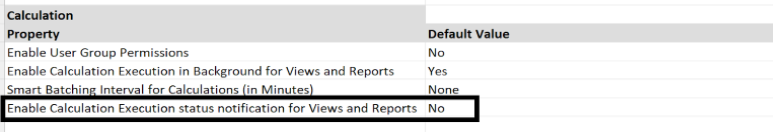
When this flag is set to YES,

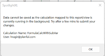
1. When a user tries to save a report/view with a Calculation mapped to it, the system checks the execution status of a calculation on the model. If it is “In Process,” it shows a notification on the status and suggests the user try after some time.
   

   Note:

   User updates are retained so the user can submit the report/view after the calculation execution is complete.

2. If the user opens a report that has a calculation mapped to it, and if there is a calculation running, the user will see a notification as below:
   

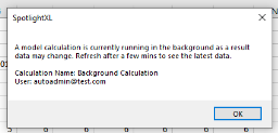
When to use this notification framework:

• This notification framework is beneficial to avoid any potential concurrency issues of simultaneous calculation executions of the model.

  • When you have multiple “save” enabled reports/views with calculations mapped to them, this option allows you to notify the users of the status and prevent frequent or simultaneous submissions.

  • When Calculations are configured to run in the background.

Dynamic Planning - Calculation Scheduler Options

The Calculation Scheduler option is now available via the Dynamic Planning Model Manager.

This Calculation Scheduler functionality offers two key improvements:

• Easily Pause and Un-Pause Schedules

• Enhanced “Repeat” schedule option to schedule calculation “Hourly”

Pause and Un-Pause schedules:

• Select the schedules (multiple or all ) via the new Calculation Scheduler

• Use the “Bulk Action” options to Scheduler On or Scheduler Off

• Use this option to administer your Dynamic Planning schedules more efficiently in a few clicks

Enhanced Repeat Scheduler option:

Now you have the option to schedule Dynamic Planning calculations at a “Hourly” frequency.

This option allows you to schedule your calculation more frequently instead of just creating at the current “Daily.” Many customers or solution architects create copies of the calculation and schedule them to run at different times daily to work around the limitation. This improvement eliminated the overhead of calculation maintenance significantly.

How to enable this “Hourly” schedule option?

• Contact Planful Support via the Support case

• Support enables the following flag for the Dynamic Planning application

  • Enable Schedule Hourly Repeat Option

FTP/SFTP native Planful connector

The native FTP/SFTP connector allows users to connect to an SFTP server, fetch data files, and load the data into Planful.

Below are some details on the Provisioning, Implementation, and Best Practices of how you think and adopt this native Planful connector.

Provisioning

1. Is this option available for all customers?
   No. This is an Opt-in. Special licensing terms are applicable for the SFTP option. Please work with the Planful account manager.
   
   

2. What process is involved if the customer has a license for the SFTP native connector?
   Customer SFTP site credentials are created and supplied by the Operations Support Team. Create a Support ticket for the SFTP setup to configure these for the customer application.

   The Support needs to enable the SFTPDataload option for the customer application by setting the following configuration flag:
   EnableSFTPDataLoads
   
   

3. What are the steps to establish an SFTP load process?
   Following are the task steps that need to be completed:
   1. SFTP server configuration
   2. Data Load Rule setup of type FTP/SFTP
   3. Cloud scheduler process flow task to automate the load at a scheduled interval
   
   

   Note:

   (Internal only note) Application must be on the new Planful framework called IVY. All new applications are, by default, on the new framework. ~ 98%+ existing customer applications are on IVY. IVY framework is not available for non-12 Period applications. If the application is not on the IVY framework, we encourage adopting the new framework for your application(s).

   Implementation/Scoping Related

4. What are the load types supported via FTP/SFTP connector?
   Currently, we support GL Data Loads, Translations, and Transaction data loads. Note that you should use the Transactions V2 data load option for the Transactions upload.
   
   

5. What is the structure of the FTP/SFTP folder?
   There will be three folders (Input, Success, and Failure) for each Data load rule of type FTP/SFTP.
   
   
   

6. What happens when the DLR folder name is manually changed at the SFTP folder path?
   Data Load simply fails. It is not recommended to manually alter the folder names or path at the SFTP site.
   

7. What happens if the Input Data Load Rule folder contains no data files?
   The data load for that Data Load Rule fails, and the details are displayed in Maintenance -> Cloud Scheduler -> Job Manager.
   
   

8. When should I position native FTP/SFTP for my customer?
   Certainly, position this for any customer looking for an option to automate their load process using a file upload; this option would make perfect sense.

   Note:

   This option automates the customer data load process with the scheduling option(s) available via the Planful Cloud Scheduler process flow.

   
   

9. Is this option more appropriate to use over Boomi?
   May not!! The Boomi-based process flow is most appropriate for customers with the following broad requirements:
   1. To automate the data extraction from the Customer source system(s)
   2. To perform advanced transformations and create mapping rules for the Planful data structures
   When a customer has these requirements, a Planful data integration specialist `performs the scoping of such work and develops a solution via Boomi-based process flow or other integration tools.
   
   

10. Are there any sort of file/data transformation or manipulations possible if we use the native FTP/SFTP option, and how do we configure it?
    Basic file transformations are available, such as column Join/Spilt/Move/Replace/Create, etc.. Configure them at the Data Load Rule level. For more information, go through the help.
    Additionally, if you are looking for translations from your local chart of accounts file to a common chart of accounts configured in Planful, leverage Planful’s Data Integration Translations functionality as you do for the regular data loads in Planful with the established translations.
    
    

11. I have a customer with Boomi - SFTP process flow. Should we consider this option?
    We are not suggesting a change to the existing process flows. Boomi flow may have more complex logic and mapping to the Planful GL mappings in a customized way. A conversion might need a substantial evaluation, planning, and change management.

    Best Practices /Guardrails

12. How many files can I configure to load via FTP/SFTP, and what are the general guidelines/guardrails?
    We can run up to 20 files of size 1 GB each. We strictly recommend “Incremental data loads” for GL and Transactions. Our Transactions V2 has support for incremental loading as well.
    
    

13. What are the file types supported?
    Planful supports importing data from .xls, .xlsx, and .csv formats.
    
    

14. How many days of History can I keep in the SFTP folder?
    We encourage implementing a periodic purging strategy. If you are loading multiple files and the load frequency is more than four times daily, we encourage removing files older than a week from the Success and Failure folders. In other situations, you can keep up to 30 days. This is to ensure we have consistent performance while connecting and loading the data.
    
    

15. Do we have an automated way of deleting the old files on a scheduled basis?
    Currently, we don’t have an automatic deletion capability from the application. It is a manual process to clear the files from the corresponding FTP/SFTP site folder path. FTP/SFTP site administrators access the folders and delete the files manually.
    
    

Insights of the Smart Batching for Calculations Mapped to Views and Reports

Calculations mapped to a View or Report can be triggered and run in the background or foreground using the flag option “Enable Calculation Execution in Background for Views and Reports”. This option can be configured from Manage > Application Settings in SpotlightXL.

When the flag “Enable Calculation Execution in Background for Views and Reports” value is set to YES, calculations will run in the background (Note: The calculation must be configured to “Run in Background” at the Calculation setup level.). It leverages the “Smart Batching Interval for Calculations”. This option can be configured from Manage > Application Settings in SpotlightXL.

When “Smart Batching Interval for Calculations (in Minutes)” is NONE,

• When a user submits a calculation, the calculation will be submitted for execution. If another copy of the same calculation is executed, the newly submitted one may fail depending on the overlap status/concurrency. Ensuring you have an optimal scoping setup for your calculations is recommended to avoid any unforeseen issues with the data due to the calculation step dependencies.

• When a user submits a calculation, the calculation will be scheduled with a specified delay time. Multiple copies of the same calculation can be scheduled, provided runtime variables passed from the view or report have different values (at least one variable). Calculations are batched using the key consisting of tenant code, model name, calculation name, and variable names and values.

• If a scheduled calculation with the same key already exists, the new request will be batched with it. Otherwise, a new calculation will be scheduled. In a heavy concurrency scenario with small calculation run times, we recommend leveraging appropriate smart batching intervals between 1 minute to 60 minutes, depending on the largest calculation run time from your report/view. Ensuring calculations are scoped with runtime variables on the key dimensions is important.

User Integration APIs Overview and Best Practices

Below is a high-level overview of various User integration scenarios of Structured Planning APIs to create/update users and user approval roles. For more information on the relevant APIs, check out this link.

Custom URL Option - Here is what you should consider

With the Custom URL/ Subdomain feature - The current URL structure will be modified to reflect a unique customer name.

For example, if the customer name is "demoabc," the new URL will be demoabc.Planful.com.

This feature is available as an opt-in for the customers, and you can reach out to Planful Support to create a Custom URL for your application.

Here are a few critical items you need to consider before initiating the customer URL process to prepare the customer admins and the users:

User Experience: Post-migration, the existing URLs “epm01.planful.com” will continue to work but without login via SSO support on the login page.

• Example: If users actively use the platform on "epm01.planful.com" and the URL changes to "demoabc.planful.com," the user will be prompted to log in again with the updated URL.

User Auth and Settings: As part of the URL change, certain Authentication and settings may be affected. This includes the loss of "Remember User Name" and "Remember Password" settings on the landing page, as well as the “reset” of cookie settings related to 2FA (Two-Factor Authentication) and OTP (One-Time Password) remembrance. Additionally, notification settings may need to be reconfigured.

• Example: After the URL change, you may need to re-enter your username, reset your password settings, and adjust your notification preferences.

API Integrations: It is important to note that the change in the customer URL will not impact API login flows, such as OAuth, Web Services, and Web API. These integrations will continue to function seamlessly.

• Example: If your organization has API integrations with the current URL, it will remain unaffected by the URL change.

Third-Party Integration: It is important to note that the change in the customer URL will not impact any integration. These integrations will continue to function seamlessly.

• Example: If your organization has any third-party integrations set up with the current URL, they will remain unaffected by the URL change.

OLH: The existing OLH (Online Help) and other static pages will not receive customized URLs and will continue to function as-is.

Migration: It would be done in a pre-scheduled window of up to 30 mins off-peak time for the migration or the update.

Insights on Reporting Currencies

Planful allows flexible reporting currency options in Structured Planning to allow the user to report at the alternate currencies (other than their Common Currency) or perform the conversion at a constant or prior year rate, etc., for the reporting/analysis.

Below are considerations while setting up or troubleshooting a Reporting Currency:

1. Ensure the Currency Exchange Rates are provided, if the Currency Exceptions are configured, check if the exception configurations have the “rate” defined. When there is no rate defined for any period, no currency conversation happens.

2. Special note on the Currency Type usage:

1. 1. 1. If the “Currency Type” for the currency conversion is set to “Not Translated (NT)”, no conversion happens. So, please check your account configurations.

      2. If the “Currency Type” is set to “SAME”, the exchange rate will be considered as “1” as a result you will see the same number after the conversion as the Local Currency.

3. A note on Opening Balance: Behavior is driven by the “Account Type” configuration. For all “Flow” accounts, at the end of the FY, balance will be reset. However, for Balance Accounts, the behavior is dependent on the following configurations:

1. 1. 1. Do Not Consider Opening Balance: When selected, Opening Balance won’t be considered.

      2. Overwrite Opening Balance: This will be applicable when you want to overwrite the Opening Balance value from the Scenario setup screen for the Planning scenarios. Otherwise, by default, the History Periods configuration will be used for the Opening Balance.

4. A note on CC Data usage in Reporting Currency computation:

1. 1. 1. Reporting Currency computation involves the following conversion steps:

         1. Local Currency to Reporting Currency

         2. Common Currency to Reporting Currency

      2. When the Reporting Currency, Currency Code (ex: USD) is same as the Common Currency (ex: USD), you may want to skip this data copy, for this you need to select “Do NOT Consider CC Data”

5. A note on CTA (Currency Translation Adjustment): By default, the default CTA configuration will be used, however, for the purposes of Cash-flow reporting, or what-if analysis, you can override this behavior by leveraging the CTA Sets capability which allows us to compute CTA on the select Accounts only. You need to define, CTA Sets to “Overwrite Default CTA” for the Reporting Currencies.

6. For the Plan or Forecast Scenario, Closed Periods, Reporting Currency Data will be recalculated during the Closed Period refresh.

7. A note on the number of Reporting Currencies and how you can process Reporting Currencies:

1. 1. 1. We can have a max of 5 Reporting Currencies.

      2. More reporting currencies may impact performance, particularly when performing the Consolidation Process.

         1. Be judicious while configuring Reporting currencies in the application. Ensure you configure Reporting currencies that are critical and necessary.

         2. And, while running a consolidation process, be judicious about what Reporting Currencies you want to include. Use the Consolidation Process user selection panel and ensure you select to include only the required Reporting currencies as part of the consolidation process.

         3. Currency Conversions process flow option also performs the Reporting Currencies computation. This would be a great option to take advantage of the Reporting currency analysis for Planning scenarios without relying on the Consolidation processing capabilities. If there is a need for the CTA type of calculation support, you may need a Consolidation setup.

Insights and Best Practices Using Opening Balance in Data Loads

Planful Data Integrations in Structured Planning application allows mapping “Opening Balance” from the source system to Planful while loading MTD-type data load. This column value will be used to compute YTD following the data principles.

With our new data fabric framework IVY, we have subtle improvements to support Opening Balance while consistently maintaining the data integrity related to the MTD and YTD balances.

In summary,

1. Be judicious in using the Opening Balance loads in your DLRs; keep the Opening Balance loads only during the beginning of the fiscal year.

2. When possible, load the YTD data loads instead of the MTD load for the Balance accounts.

Number Formatting Ideas on Dashboard Tables with Custom or Calculated Members

We can present alternate column or row-level number formatting for your Dashboard tables to represent your key metrics with the following method.

In the below example, we have $ and % representations made in the Dashboard table views.

1. To represent the % format on the dashboard view, create the calculated member or custom member below with a type cast as String and concatenate with “%”

   • CStr(CInt(([Account].&[304]/[Account].&[216])*100))+"%"

2. If you need to apply the variance-based calculations for Actual to Budget variance for the same metrics, create custom members on the scenario dimension with the expression below to force the account in context for the % format.

   • IIF(Account.CurrentMember is [Account].&[993],
     CStr(CInt((([Account].&[304],[Scenario].&[1])/([Account].&[216],[Scenario].&[1]))*100 - (([Account].&[304],@CURBDGT@)/([Account].&[216],@CURBDGT@))*100))+"%",([Scenario].&[1]-@CURBDGT@)
     )

This method is to show you the custom member or calculated member capabilities with our dimensional member-based expression.

Zoom to Data Leaves for Excel Analysis Views is available now for Direct Access to Planning Models.

Support for the Zoom-in -> Data Leaves option allows you to query your Direct access planning models much more efficiently without going through the number of clicks.

When you zoom in on large dimensions like Project or Client, you may experience challenges seamlessly navigating to the members with data. This limitation has now been addressed with our new Data Leaves option for Excel Analysis Views built for Direct Access to Planning for efficient querying for the dimension members with the data when you Zoom in.

Currently, this feature is available as an opt-in with a flag (Enable Axis Query API flag). This option will become available as a standard feature in the upcoming releases.

Optimizing the DownloadData Calc Performance with Periodic Maintenance of Financial Model

Do you know periodic maintenance of the Finance model (HACPM_Financial) would help your overall calculation performance involving DownloadData step? In a customer situation, we have seen their performance improve by over 40% just by the Clear model on HACPM_Financial.

Depending on the design and requirements for housing the data in HACPM_Financial, we recommend introducing a maintenance process to keep only relevant data in the HACPM_Financial.

You can employ the following 2 approaches

1. Clear Model from Model -> Setup screen. Using this Clear Model option on the HACPM_Financial clears all the data, and your model will still be in the Generated state. With this method, your HACPM_Financial will be cleared entirely and in that state until you run the DownloadData step via your Calculation.

2. ClearAllModel Calculation Type with Scope. This will help you selectively clear the data and retain the required data within the HACPM_Financial by applying filters on Scenario, Time, and Measures.

Use this data maintenance process to ensure that you have consistent performance with the DownloadData step and the DP calculations.

Incremental Cube Processing Insights

Do you know Incremental Cube Processing happens even without your application's Automated Data Refresh (ADR) option turned ON? Read below to know how?

Do you know we can control the frequency of Automated Cube processing events in your Job Manager with the Automated Data Refresh (ADR)?

Incremental or change-only data processing for Cube helps see the data faster in reports. And the performance of the Incremental processing will be significantly faster than the Full process. In most cases, improvement will be ~4X.

Here are some key insights into this capability

• Our data processing framework IVY made Incremental processing functionality possible by tracking the data changes across our data sources like Templates/DLRs etc. Learn more about IVY here! At the time of writing this, we have approx 70% of applications on the IVY framework.

• As IVY continues to track the delta changes across all your data sources like Templates, Journals, or the Data Loads, when a user triggers the cube process manually, if there is a delta available, Cub processing will be performed automatically in the “Incremental” processing mode rather than the traditional “Full” process model This gives you a significant advantage. So irrespective of the ADR option, you can take advantage of the “Incremental” processing. The only pre-requisite here is - the application should be running on IVY.

• With the Automated Data Refresh (ADR) option, you can automate the cube refresh process so you can see the data after the template changes or journal postings. See more information on Automated Data Refresh here! However, depending on the template activity rate, data loads or journal posting, etc.., you may see a continuous stream of automated cube-processing events. This situation will likely impact your report performance and have too many cube processes in the Job manager! This situation can be optimized by leveraging a “Wait time” configuration.

When to consider ADR “wait time” configuration?

• If you start to see frequent cube process events in the Job manager (every few seconds).

• or, if your report users experience lag in the report run times. If you see a longer run time on key reports if you run them right after the cube processing event!

How this ADR option of “wait time” works?

• A value to this flag specifies the number of seconds (say 600 seconds) the cube processing task is to be delayed! Any duplicate requests will be discarded while a task is processed or in Queued State.

• This option is available only if the application is fully on the IVY framework.

How to get this ADR option of “wait time” enabled?

• Contact Planful Support via the Support case.

• Support adjusts the flag value in the seconds (say 600 seconds / 1800 seconds)

  • Debounce WaitTime

Option to Optimize the DLR process when you have multiple Writeback steps in the Dynamic Planning Calculation

By definition, it is not recommended to have the Same Data Load Rule used in the multiple Writeback Map Steps in the same calculation; However, if you have to use it for any specific situation, you can optimize the load behavior using the following option.

• Consolidated Writeback

When to consider this option?

• When the same DLR ID is referenced for the Writeback ID of the different Map Steps listed on a Calculation

How does this work and improve the performance?

• Data from all writeback steps are accumulated and then written back to Structured Planning once all the calculation steps have been completed.

What happens if there are multiple DLR IDs in the same calculation across different maps?

• Accumulated data is written back to Structured Planning separately for each DLR.

How to get this enabled?

• Contact Planful Support via the Support case.

• Support enables the following flags for the Dynamic Planning application:

  • • Enable New Writeback Features

    • Enable Consolidated Writeback