Cell Level Formatting Explained

3 Minutes to read

Print
Dark

Light
PDF

Article summary

Did you find this summary helpful?

Thank you for your feedback

With Cell Level Formatting, you to control the look and feel of report output down to the cell level. Apply formatting to the entire report, a row/column, a range of cells, or an individual cell. Additionally, you can:

apply formatting when using the insert formula row/column in a report
format a formula exception value
vertically top/center/bottom align headers and numbers in a report

Note:

Header and Footer rows honor the formatting applied from the Header & Footer section

If you opt-in, this functionality applies to all existing and new Dynamic Reports across all browsers. It is available for all reporting areas (Financial, Sales, Workforce).

Cell Level Formatting is enabled for Dynamic Reports that are designed using dimensions or attributes and Report Sets on the Row or Column axes.

Note:

The Cell level formatting options in Dynamic Reports are enabled by default for new and existing tenants.

The default format for a Dynamic Report is:

Column headers are center aligned and bold
Row headers are left aligned and bold
Drill down members are shown with indents
Numbers are right aligned
Font = Arial, size = 8, color = black, fill color = no color

Formatting is applied to all cells within the body of the report and:

Applies to row and column headers, numbers/data values in the report
Applies to merged cells (when multiple dimensions are used on the column axis)
Notes, Insert Formula row/column, Formula Exceptions

Formatting is retained when exporting a Dynamic Report, when it is included as an email attachment, linked report, and when used in a Report Collection or FPP.

When the structure of the report is modified by adding or removing dimensions from the row or column axis, formatting has to be readjusted for accuracy.

In Practice

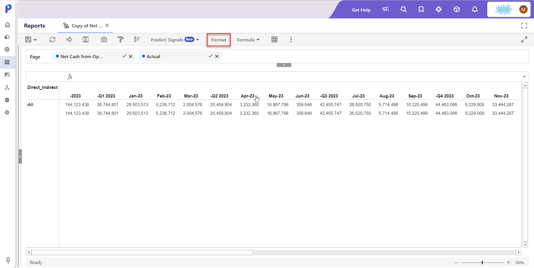
To apply cell level formatting to a Dynamic report, open the report, and click Format (an example is shown below).
The Format pane appears. There are 3 tabs; Text, Data, and Other. Ensure the Text tab is selected.
Select a cell and apply different styles. The same report shown above has been modified.
To select a range of cells, drag the cursor as you would in Excel.
Change the font type and size.
Planful supports a range of font types, which are enabled in Static Report Sets. Select the list-box to view all supported font types. Fonts size 8 through 32 px are supported. The default is set to 8 for all existing and new Dynamic Reports across all the lines. Based on the font size the row height automatically adjusts.
Select alignment and indentation options.
Apply borders to the report. Select a cell or cells, select a border color, and click the border type to be applied.
Here is the border color and border type selection pane. There are many options to choose from including, no border, left and right border, and top and bottom border.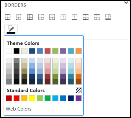
Click the Data tab.
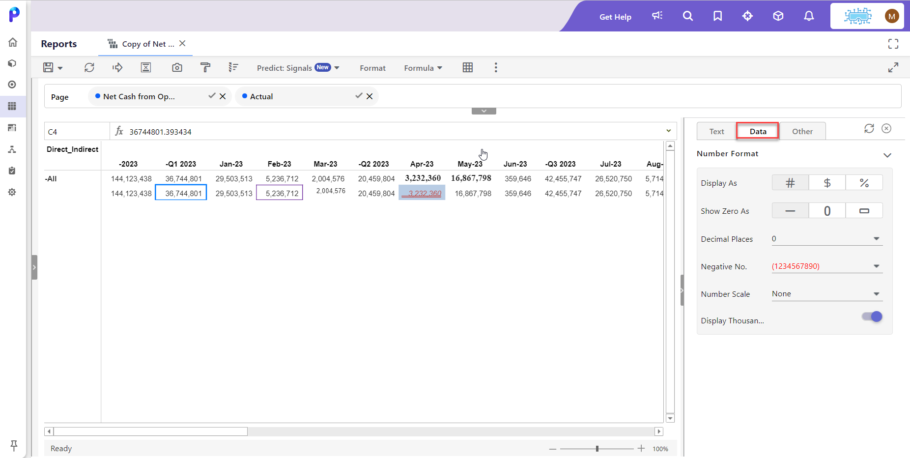
For Display As, select to display the cell contents in number, currency, or percentage format. When currency is applied to a cell or cells, the Currency Alignment options displays as shown below.
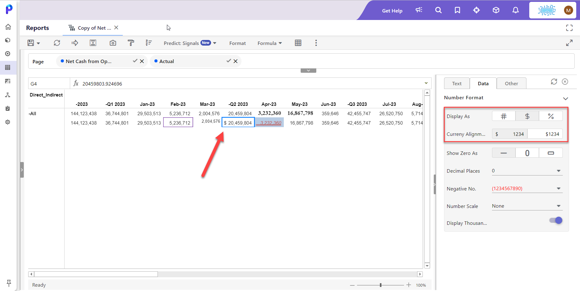Select how you want the currency symbol displayed in the cell. There are two formats; Accounting and Currency. With the Accounting format, the currency symbol is displayed in the left-most position within the cell. With the Currencyformat, the currency symbol is displayed directly in front of the number in the cell.When multiple formats are applied to the report, only the most recently applied format gets applied to each cell in the report. When multiple cells with different formatting are selected, format of the first cell is displayed in the pane. Formatting is not supported when Properties are added to the report.
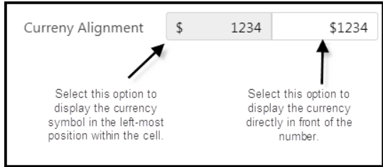The Currency symbol displayed is based on your location settings.
For Show Zero As, select how you want to display zero values (as dashes, empty, or as 0) for a selected cell, cell range, or the entire report. Selecting 0 applies to all data values in the report including, Excel calculations, insert formulas, and formula exceptions.
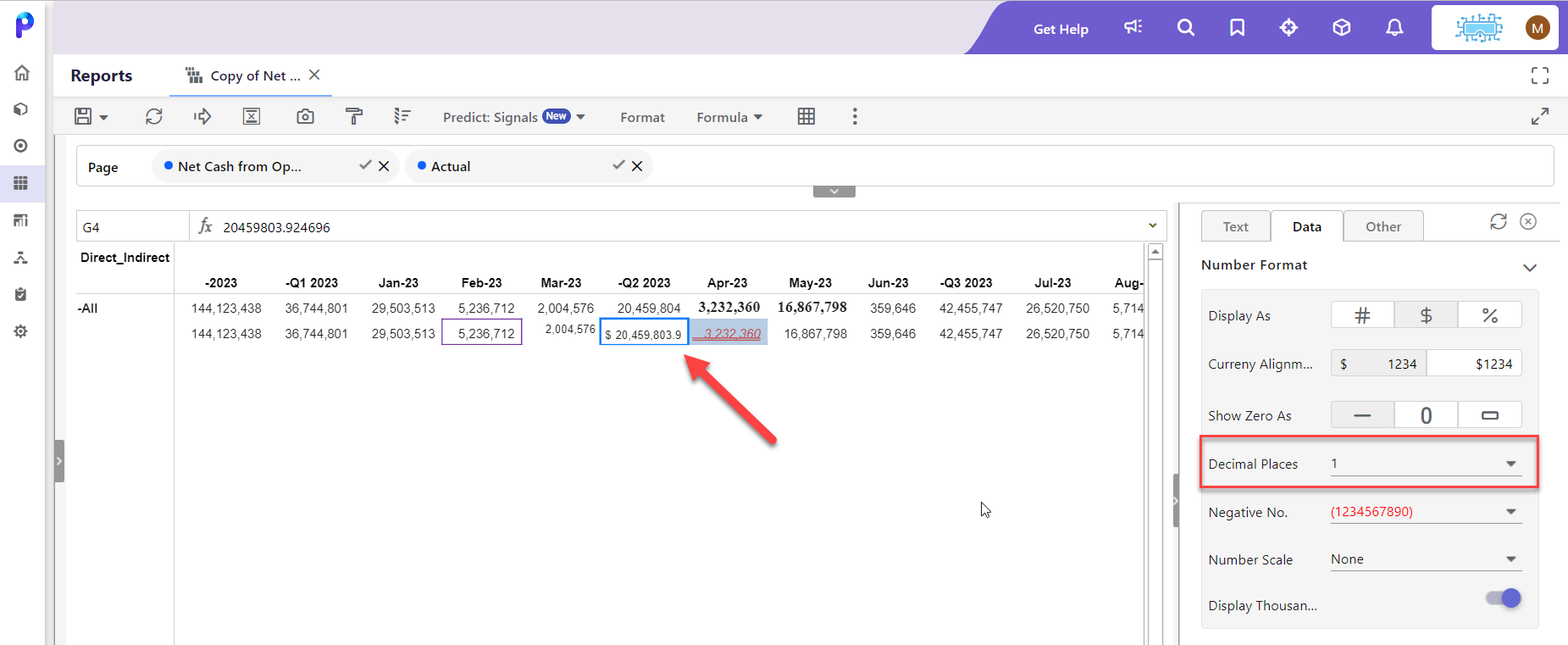
Select the number of decimal places for a selected cell, cell range, or report. In the example below, 1 decimal places is selected for a cell. You can select 0 to 6 decimal places.
Select a Thousand Separator option. Display of the thousand separator is driven based on user location settings.
Finally, click the Other tab and select to hide or display empty rows and columns. Don’t forget to click Apply and Save!

Was this article helpful?

What's Next

How to Reset Formatting Selections