Dynamic Planning: Aggregation Process

Effective aggregation techniques provide more information based on related data clusters, such as a company’s revenue or performance. For example, a store may want to look at the sales performance for different regions to aggregate the sales data based on a region.

Aggregation can be applied at any scale to summarize information and make conclusions based on data-rich findings. Data can also be aggregated by date, showing trends for years, quarters, months, etc. These aggregations could be placed in a hierarchy, where you can view the data trends for years, then see the data trends over months for each year.

Aggregation

An aggregation function is a mathematical computation involving a range of values that results in just a single value expressing the significance of the accumulated data it is derived from. Aggregate functions are often used to derive descriptive statistics. For example, an aggregation function groups together the values of multiple rows as input on certain criteria to form a single value of more significant meaning.

Improvement and Business Value

The Aggregation algorithm has been enhanced to process the data quickly and accurately, saving a lot of time working with large data models. Previously, the Aggregation algorithm used to take a considerable amount of time to process the data. For example, to process all data records in a model with 10 dimensions where 6 were Key Dimensions and 4 were Value Dimensions, the Aggregation algorithm previously took close to 18 minutes. With this release, the Aggregation algorithm will process the same data records in just three and a half minutes. This significantly reduces the time and greatly increases the performance of the process.

The processing time depends on the key and value dimensions, rollup operators, dimensions and levels within each dimension, and the total number of records in the model. The algorithm is much more optimized in computing the rollup values in the model hence users will see that it's taking less time to complete the aggregation.

With the Aggregation algorithm, the overall time it takes to complete the aggregation will be cut down to half. We have tested the aggregation algorithm with various models and in all these tests the aggregation times have improved in some cases.

Performance Improvement Use Cases

Example 1: A model of size 3770.90 MB has 10 dimensions where 6 were Key Dimensions, and 4 were value dimensions. The following table shows some data of the data processed and the time consumed for aggregation.

With the old aggregation algorithm, the time consumed for aggregating the same model was 18 minutes 22 seconds.

Example 2: A model of size 18300.4 MB has 9 dimensions where 5 were Key Dimensions, and 4 were value dimensions. The following table shows some data of the data processed and the time consumed for aggregation.

The time consumed for aggregating the same model was 36 minutes 55 seconds.

Example 3: A model of size 6698.2 MB has 6 dimensions where 3 were Key Dimensions, and 3 were value dimensions. The following table shows some data of the data processed and the time consumed for aggregation.

The time consumed for aggregating the same model was 2 hours 45 minutes 54 seconds.

Enable Aggregation Performance Flag

You must contact the customer support team to enable the aggregation performance flag in your application.

Once the aggregation performance flag is enabled in your application, perform the following:

• Log into your application.

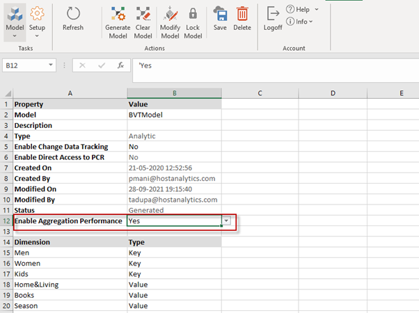
• Go to the Model Setup screen, and set the ‘Enable Aggregation Performance’ property to ‘Yes.’

This property can be enabled even for models with Change Data tracking enabled; that is, the aggregation performance improvement can be enabled irrespective of whether the model has Change Data tracking or not.

If you have multiple models in the application and need to enable aggregation performance for all models, one option is to manually enable it from the Model setup screen. Another option is to request the support team to enable it from the backend.

Once you enable the flag in the Model screen, the Aggregation function will run the algorithm. You can choose which model you want to enable for the same Tenant.

This change enhances the Aggregation Performance and significantly reduces the time previously taken for aggregation.

In Practice: To enable the Enable Performance Flag in SpotlightXL

1. Open SpotlightXL, and go to the Model Setup screen.

2. Now, navigate to the Enable Aggregation Performance property, and select Yes from the drop-down options.

Structured Planning, Consolidation, and Reporting Applications Download Script > Model > Calculations

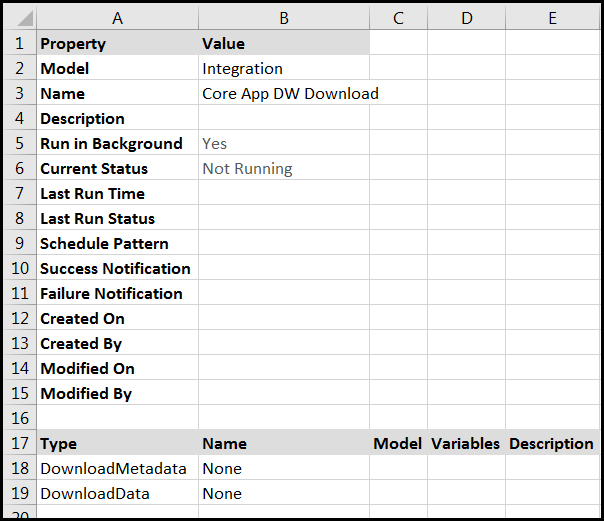
Give the calculation a name: Core App DW Download. This script will refresh HACPM_Financial with the latest metadata and data from the DWMaster database in the Structured Planning, Consolidation, and Reporting applications. Remember, you used the Application Settings page to specify that Dynamic Planning should connect to the DWMaster database in Structured Planning, Consolidation, and Reporting applications.

In Practice

1. Set Run in Background to Yes.

2. Enter your email address in the Success Notification and Failure Notification fields.

3. Under Type, add two commands using the drop-down: DownloadMetadata and DownloadData. Under Name, type None.

4. Then Save the calculation.

   

Model Refresh Script > Model > Calculation

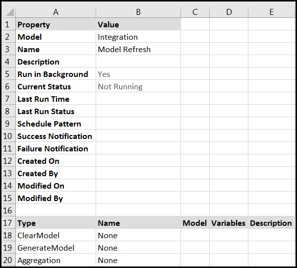
Now create another calculation called Model Refresh. This script will clear all existing data from the model, load data from HACPM_Financial (via Generate Model), and run an aggregation.

In Practice

1. Set Run in Background to Yes.

2. Enter your email address in the Success Notification and Failure Notification fields.

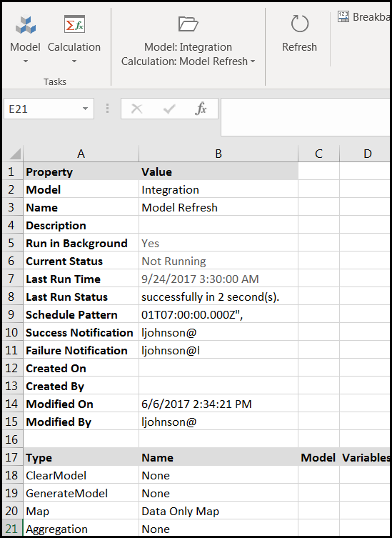
3. Under Type, add three commands using the drop-down: ClearModel, GenerateModel, and Aggregation. Under Name, type None.

4. After creating the calculation, be sure to Save it.

   

Running a Data Map Explicitly

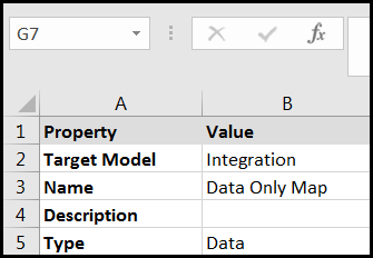
If you previously specified a Map of type Data (see “Generate Model ” above), you need to explicitly run the map in order to copy data into your model.

In Practice: Model > Calculation

1. Give the calculation a name: Run Data Map. Then specify under Type that it should run a Map, and then provide the map name.

   

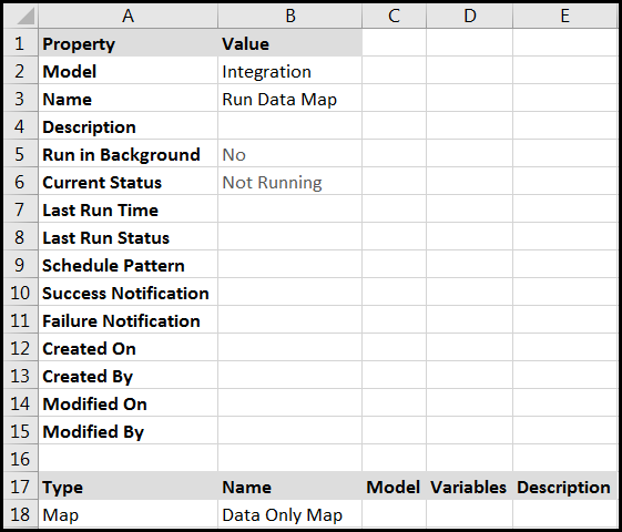
2. Then Save it.

3. To run the map during model refresh, add the Map line to your Model Refresh calculation.

   

Scheduling Download and Refresh Scripts

Power or Contributor user access is required for these steps.

When Dynamic Planning is used for analysis and reporting on data from Structured Planning, Consolidation, and Reporting applications, data needs to be refreshed in Dynamic Planning on a regular basis. You can schedule the Download and Refresh calculations to run regularly, such as overnight.

You can schedule daily, weekly, or monthly runs.

In Practice: Model > Calculation

1. Select the model and calculation that you want to schedule.

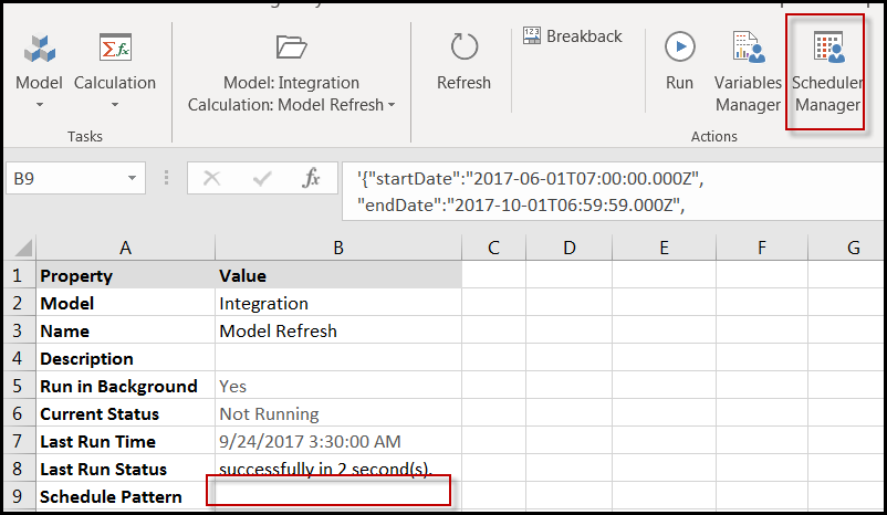
2. Select the cell next to Schedule Pattern and then click Scheduler Manager.

   

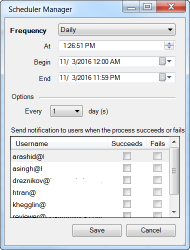
3. Click to put checkmarks under Succeeds or Fails email next to the Power user’s username.

4. Specify the time you want the calculation to start running in the At box.

5. Specify how many times you want the calculation to be run by selecting Begin and End dates in the Interval section. By default, the dates also have times denoting the beginning of the Begin date and the end of the End date. In the example below, the calculation will run at 2 AM daily from April 1 to May 1, 2016. That is 2 AM according to the clock on the server, so Power users should be aware of the time zone of their server when setting the start time. Then click Save.

   

The Schedule Pattern cell is now populated with coding about the timing of the auto-calculation.

The dates and times are shown in UTC (Coordinated Universal Time) time format.

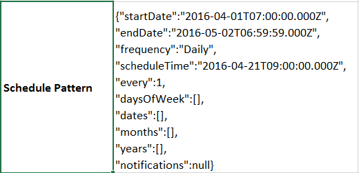
After changing the Schedule Pattern setting in the calculation, you must save the changes to the calculation also.

After setting the schedule for Structured Planning, Consolidation, and Reporting applications Download, Power users may want to then schedule the Model Refresh for an hour later. Or put all the commands from both calculations into one calculation and schedule it for an overnight run.

After the calculation is run, Last Run Time and Last Run Status are populated.

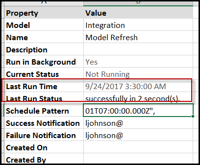
Dynamic Planning sends a notification email to state whether the calculation was successful or not.

You can also select Manage > Application Administration > Request Status to see the status of the calculation run.

Using Substitution Variables with the HACPM_Financial Model

You can define substitution variables on the HACPM_Financial source model. The variables can then be used in calculations and maps to more fully automate data loading from Planful applications.

In Practice: Define a Substitution Variable on HACPM_Financial

1. Select Model > Model Administration > Substitution Variables.

2. Select HACPM_Financial from the Model drop-down.

3. Specify which dimension will have the variable from the Dimension drop-down.

4. Provide the substitution variable name and value in the table.

   

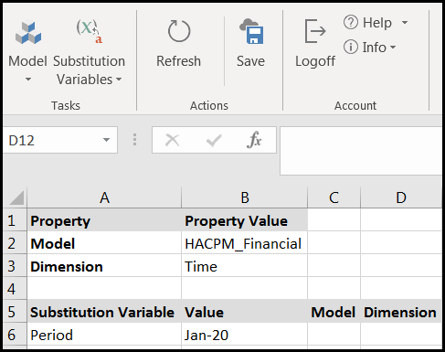
5. Click Save.

In Practice: Using the Substitution Variable in a Calculation:

1. Define variables in the Map.

   

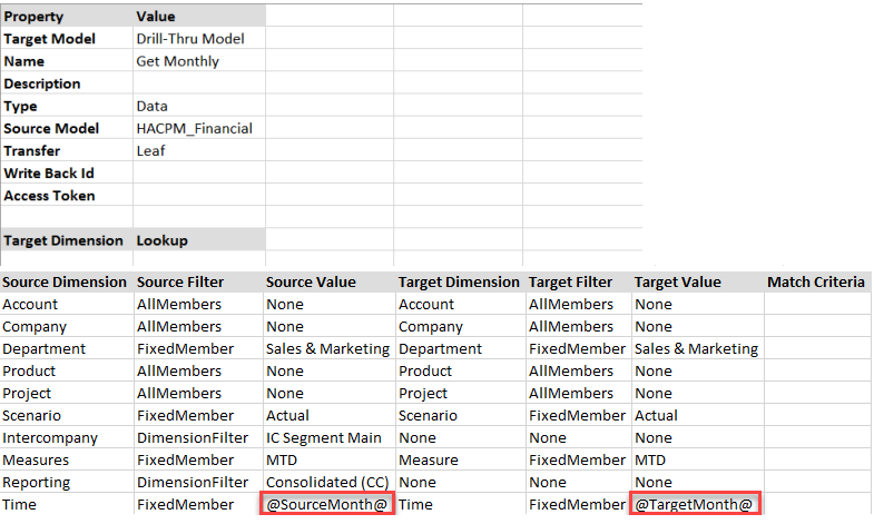
2. Use the Period substitution variable, and the SourceMonth and TargetMonth variables, in a calculation that runs the map.

   

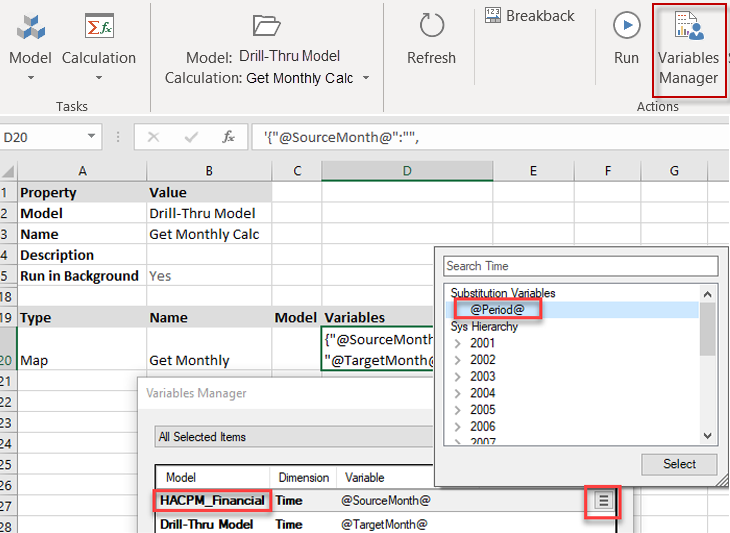
3. Each month, you simply set a Period to the current month and then run the calculation.

In Practice: Optimizing Your Monthly Data Download:

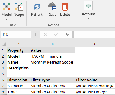
1. Define a scope on HACPM_Financial using variables that will limit the amount of data that needs to be downloaded.

   

2. Update your model refresh calculation to download only the data that is needed. In other words, download the data defined by the scope.
   

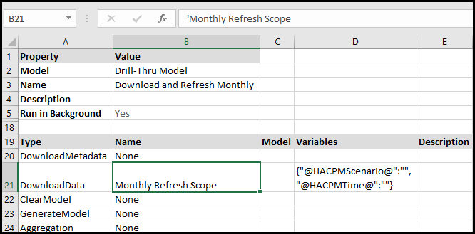
3. Select the Variables cell and click the Variables Manager button.

4. Under HACPMScenario, select the Scenario you want to view

5. Under HACPMTime, select the @Period@ substitution variable.

   

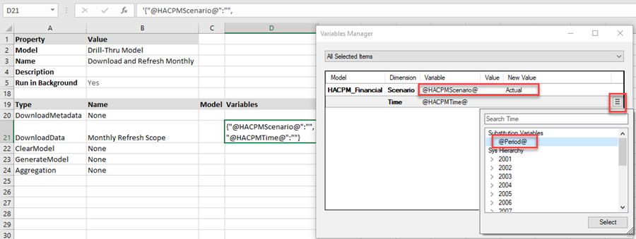
6. Click Update then Save.

7. Each month, you simply set a Period to the current month and then run the "Download and Refresh Monthly" calculation.