Transferring Data from One External Source Model to Another External Source Model

Overview

Modeling supports copying data from one External Source Model to another External Source Model. Just as you can copy data from an External Source Model into a Master or Analytic model using an ESM map, you can use the same method to copy data from one ESM to another. You must first define both the Source and the Target ESMs using the Source Model page, then you can define the Source Map to transfer the data. When the map is run, all data in the Target ESM is deleted before the data transfer from the Source Model is done.

A common use case for this feature would be to store your data load inputs in one ESM and your calculated/formula fields in a second ESM. The formula fields in the second ESM depend on data from the first ESM, so you can copy the requisite fields to the second ESM, which automatically calculates the formula fields. After verifying the data load, then load the data from the second ESM into your Master model.

Example Source ESM

In the examples in this section, the Source Model is Budget. The Source Model has 8 fields.

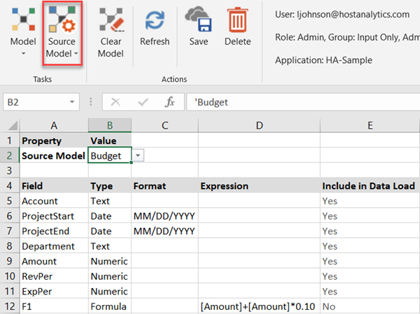
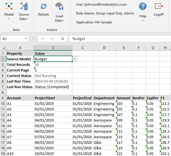
Here is the data in the Source Model.

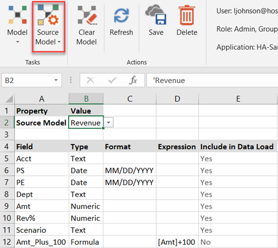
Example Target ESM

In the examples in this section, the Target ESM is Revenue. The Target ESM also has 8 fields but some fields are different than the Source Model.

Defining a Map from a Source ESM to a Target ESM

The Source Model is a two-dimensional table of data organized into fields. The Target ESM must contain at least as many data-input fields as the Source Model. You will map the fields from the Source Model to the fields in the Target ESM. You must provide a mapping for all the data-input fields in the Target ESM; data-input fields are those marked as Yes for Include in Data Load.

1. Go to Model > External Source Model > Source Map.

2. Enter a name for the map.

3. From the Model drop-down list box, select or specify the name of the Target ESM you want to map the Source ESM to. In the drop-down list box, the ESMs are listed separately under a sub-heading called ESM.

   

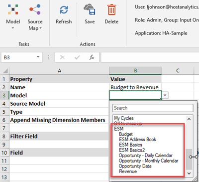
4. Select the Source Model from the Source Model drop-down.

5. Select Data for Type.

6. Set Append Missing Dimension Members to No. This option applies only to mapping to Master or analytic models.

7. The Filter Field is optional. When filters are defined in an ESM to ESM map, only the filtered data is moved from the source ESM to the target ESM. For example,let's say a filter is defined on a Department Segment field and Dept1 is the value. When this map is executed from a Calculation, the map will only move the Dept1 data from source ESM to target ESM. Additionally, the Dept1 data only in the target ESM will be cleared before the data is moved from source to target

8. Now specify the fields from the Source Model that map to fields in the target ESM. Not all fields in the Source must be mapped, but you must provide a mapping for all the fields in the Target ESM that are marked as Yes for Include in Data Load.

9. For fields in the Target ESM but not in the Source Model, specify Field: None, Maps To: DimensionFilter, the field name in the Target ESM under Target Field, and the text, number, or date to be placed into the target model under Default Value.

   

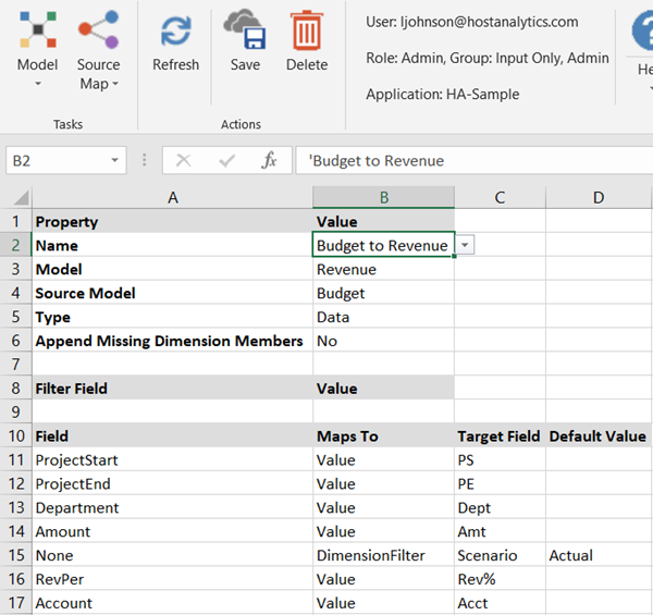
10. Save the map.

Using a Calculation to Load Data into the Target ESM

To copy data from the Source Model to the Target ESM, you must use a calculation to run the External Source Map. When the map is run, all data in the Target ESM is deleted before the data transfer from the Source Model is done, if there are no filters defined in the map. If there are filters defined in the map, the data in the target ESM will be deleted based on the filters and the source data will also be filtered based on the filters defined.

Calculations are stored within a Master or analytic model. We suggest that you create the calculation inside the Master model that the ESM data will eventually be loaded into.

1. Go to Model > Calculation.

2. Select the Master model associated with your ESMs from the Model drop-down.

3. Give the calculation a name.

4. Create the first step of the calculation by selecting ExternalSourceMap from the Type drop-down.

5. Select the name of the map you created in the previous task from the name drop-down.

6. Save the calculation.

7. Run the calculation.

   

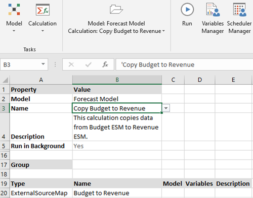
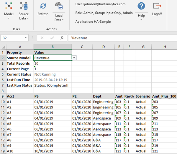
When using this calculation to execute the ExternalSourceMap, the existing records in the Target ESM are deleted, and then records from the Source Model are copied to the Target ESM. To verify the data in the Target ESM:

1. Go to Model > External Source Model > Source Data.

2. Select the Target ESM from the drop-down and click Refresh.

   If there were any formula fields in the Target ESM, they are calculated and displayed on the screen.

   

Using Filter Fields to Limit the Data Load

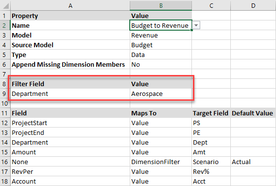
If you want to load only a subset of data in the Source model, use the Filter Field section of the Source Map to indicate which rows of data to load. In the following example, the map indicates that only rows with Department Aerospace should be loaded from Budget to Revenue.

Here is the resulting data.

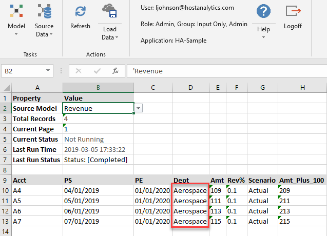
Formula Field added to Filter Fields in Maps

Formula fields are also available as filter fields in the ESM Maps. You can apply the Formula fields as filters while moving data from one External Source Model to another External Source Model, Master, or Analytic Model.

For example, if you want to load only a subset of data based on a specific calculation in the Source model, use the Filter Field section of the Source Map to indicate which rows of data to load. In the following example, the map indicates that only rows with Department Aerospace that have the Project End as 02/01/2020 should be loaded from Revenue to Budget. In this example, Department is a Text field, and Project End is a Formula field.

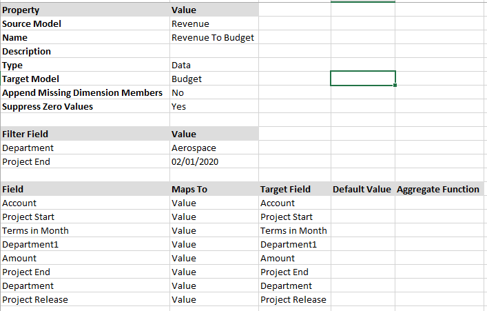
Once you run this Map, the data corresponding to the Aerospace Department with Project End as 02/01/2020 is segregated in the output.

Here is the resulting data.

To move data from the source ESM to target ESM you must create a calculation and then run the External Source Map. For more information on creating a calculation, see Run Calculation with a Map.

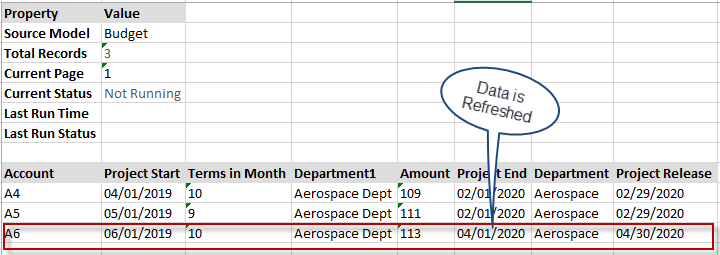
When a map is run, Reverse Filtering is applied to preserve all existing data in the target ESM that does not satisfy the filter condition. So, when you select formula filters in the map, the data that meets the filter condition will be appended to the existing data in the output.

For example, if you want to load data only for the rows of the Aerospace Department that have the Project End calculated as “04/01/2020”, you have to update the filter field in the Map as shown in the image below.

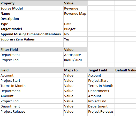
In the following example, you can see that only rows with the Department as Aerospace and that have the Project End calculated as "04/01/2020" are loaded from Revenue to Budget and appended to the data existing in the output.

Business Example

Below is an example of data mapping from an ESM to an Analytical Model. Here, you can load the rows with Gateway Cycle as the Customer Full Name field value. The data can be loaded from Purchase Information to Outline Purchase Information.

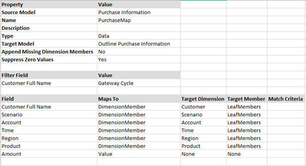
Here, Customer Full Name is the formula field that should be mapped to the Customer field in the Target dimension. The formula condition being:

CONCATENATE ([Customer First Name], “ “, [Customer Last Name])

To move data from Purchase Information to Outline Purchase Information, you must create a calculation and run the Purchase Map. For more information on creating a calculation, see Run Calculation with a Map.

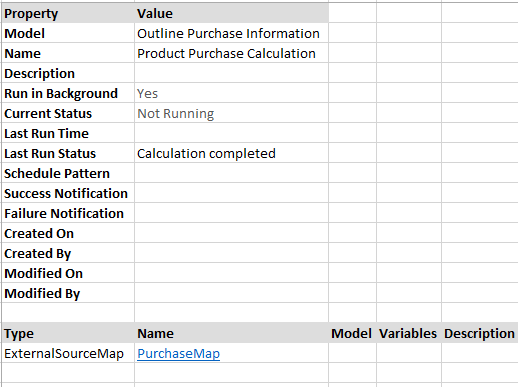
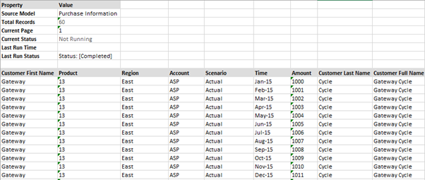
Based on the Calculation, rows with the Customer Full Name as Gateway Cycle are loaded from the Purchase Information to Outline Purchase Information and appended to the data existing in the output.

So, when you run the calculation and select the Scenario Dimension as 13, the uploaded data corresponding to the Gateway Cycle as the Customer’s Full Name Product will be updated in the output.

Business Value

With formula filters in the maps, you have the flexibility to transfer Formula field-specific data from one ESM to another instead of copying all the existing data.

It significantly reduces the effort and time previously involved to segregate data based on Formula fields and enhances the existing filtering with more options to group data.

In Practice: To use Formula Field in Maps

1. In SpotlightXL, select the Model task and the Map subtask.

2. Select the name of the Source Model defined on the Source Model page.

3. Enter a name for this map and add the description.

4. Select the type as Data for loading external source data.

5. Select or specify the name of the ESM you want to map the Source ESM to.

6. For Append Missing Dimension Members , select No when mapping to another external source model.

7. For the Filter field, specify the name of the field in the Source ESM to filter the data you want to load. Under the Value column, you can specify the value name.

8. Specify the name of the formula under the Filter field and the value.

9. For the Fields column, specify field names from the Source Model that will be mapped to fields in another model.

10. Select any of the following in the Maps To column:

    • DimensionFilter : This filter indicates that there is no field present in the Source ESM to map to the Target ESM. You will have to specify a value in the Default Value Column.

    • Value : indicates that this field in the external source is a value to be copied as is to the specified field in the target ESM.

11. In the Target Field column, select the name of the field in the target ESM.

12. In the Default Value column, specify the text, date, or number to be updated into this field.

    For information on the steps to create an ESM to ESM map and run a Calculation, see the Transferring Data from One External Source Model to Another External Source Model topic.

Filtering Data with ESM Filters

You can filter data with ESM filters in the application.

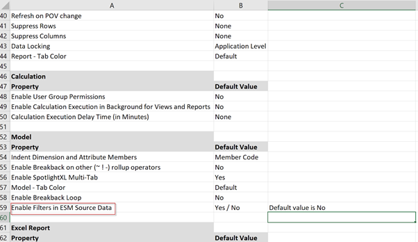
You must set the 'Enable Filters in ESM Source Data' to yes to filter data.

When you enable the flag, you can see the 'Include in Filters' column in the source Model screen. To provide value for the filter, you can either copy-paste or type the value. Also, you can only enable the Include in filters column for a maximum of 5 fields.

In Practice: Enabling the Filter Flag

1. In SpotlightXL, select the Manage screen.

2. In the Application settings drop-down, select Application Administration and then click on Application Settings.

3. Scroll down to enable the 'Enable Filters in ESM Source Data' flag. The value for this flag is set to ‘No’ by default.

In Practice: Filtering data in Source Data load

1. Select the Model task, and from the Source Model drop-down, select Source Model.

2. Define Source Model Name in the Source Model page.

3. Define Field and type in the Source Model page and click Save.

4. You will see the 'Include in Filters' column available.

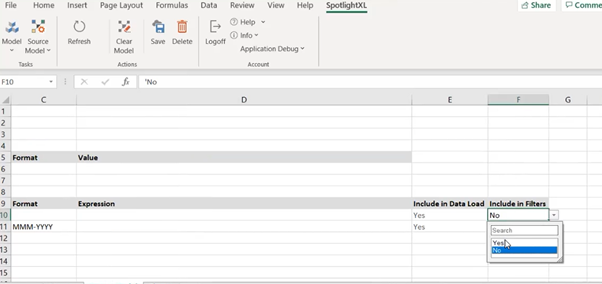
5. You can set this column value to ‘Yes’ for the specified fields.

In Practice: Loading data in the Model

1. Select the Model task, and from the Source Model drop-down, select Source Data.

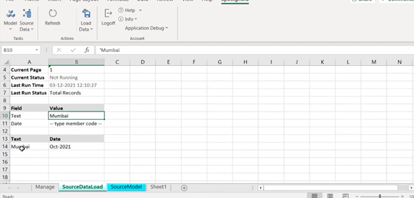
2. You can either copy-paste the values or enter them manually to load the data.

3. For the Filter field, specify the name of the field in the Source ESM to filter the data you want to load. Under the Value column, you can specify the value name.

4. After you refresh the page, you will see the filtered data based on the specified field.

Multi-ESM Use Case

The following example shows how you can use multiple external source models to generate valuable forecasting data for sales and consulting revenue.

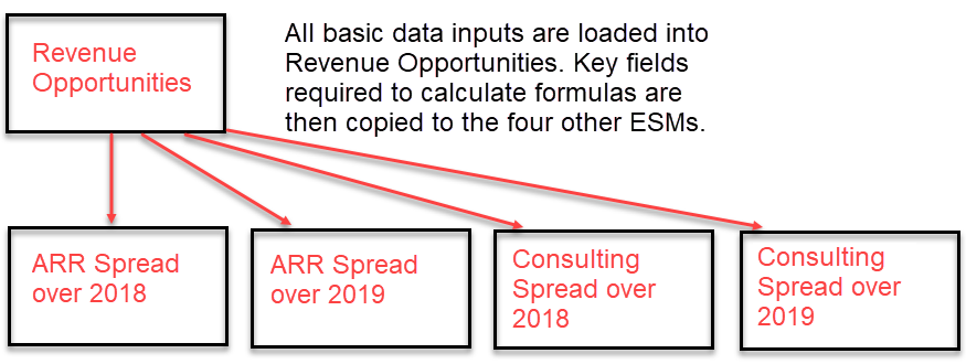
• Data inputs about the prospective customer, sales rep, potential revenue amount (ARR), and potential implementation consulting revenue are loaded into an ESM called Revenue Opportunities.

• Sales revenue is forecast monthly based on a project start date and a term. To keep the ESMs organized and of a manageable size, there is one ESM for each year to store the monthly forecast.

• Consulting revenue is forecast quarterly based on a project start date and four quarters of payments. To keep the ESMs organized and of a manageable size, there is one ESM for each year to store the consulting forecast.

Revenue Opportunities identifies 8 data input fields that you need to load.

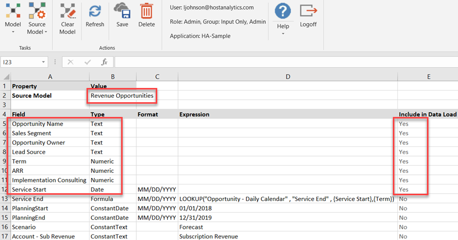
Here is the data load file for Revenue Opportunities.

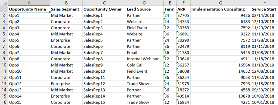
The Revenue ARR amount is spread over 2018 and 2019 in this example. An ESM for each year is created. Only 4 fields from Revenue Opportunities need to be mapped to the ARR Spread models to generate the monthly forecast.

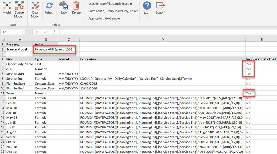
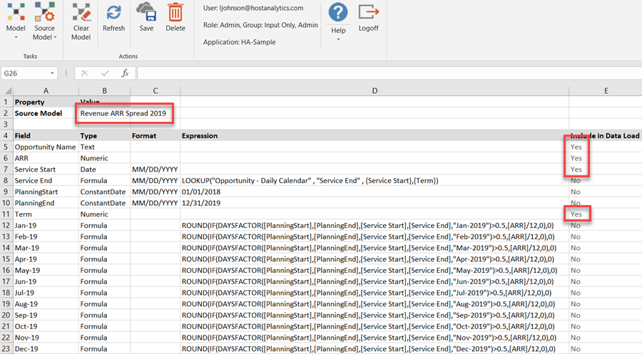
Here are the maps to copy the four input fields from Revenue Opportunities to the Spread models.

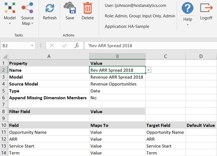
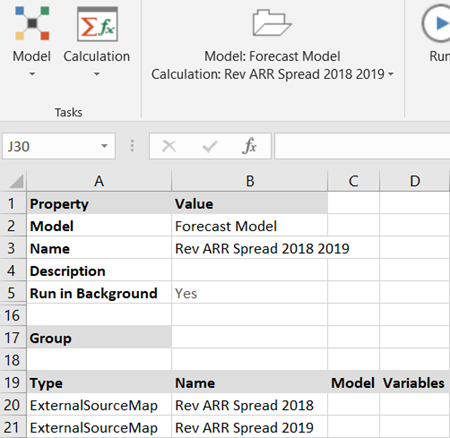
Here is the calculation to run the two ESM maps.

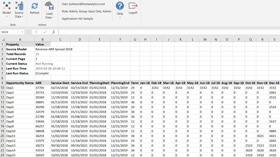
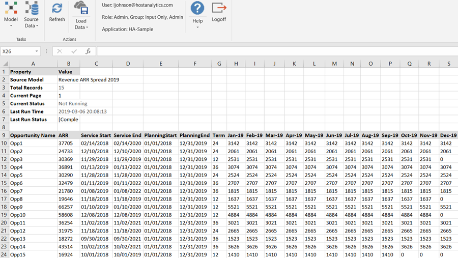
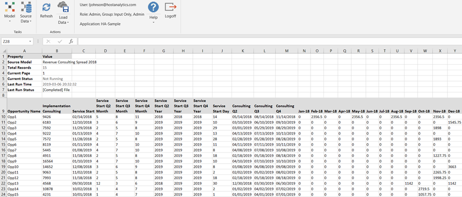
The resulting ARR spread data is as follows. For details on how the DaysFactor function works, see Explanation of the DaysFactor Function.

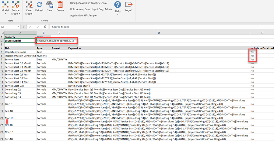
Similar to ARR, the Revenue Implementation Consulting amount is spread over 2018 and 2019 in the following example. To show a different use case, we assume that consulting will be paid in 4 equal quarterly payments and will last no longer than 4 quarters, even if the Term of the project is more than 12 months. An ESM for each year is created. Only 3 fields from Revenue Opportunities need to be mapped to the Consulting Spread models to generate the monthly forecast.

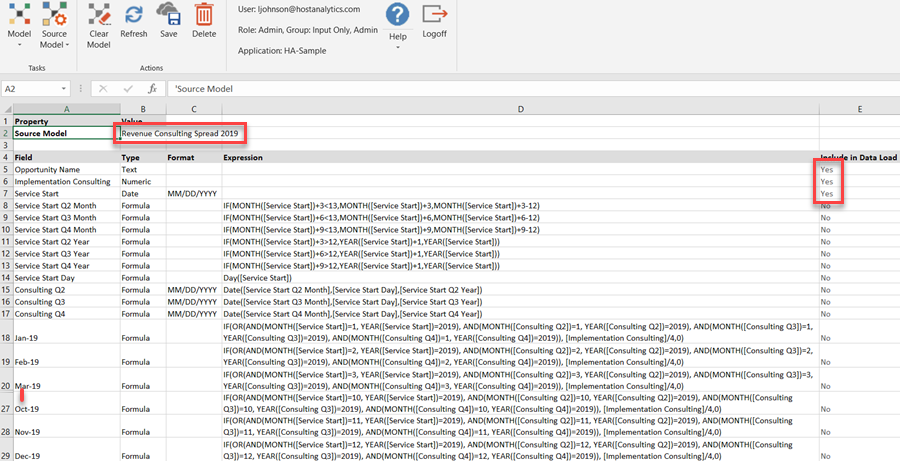
Explanation of the Quarterly Formulas

For syntax of the ESM functions, see External Source Model Field Types, Expressions, and Formulas.

• We have a Service Start date and need to calculate the dates of the following three quarters.

• Formulas are created which calculate what the month and year is 3 months later, 6 months later, and 9 months later.

  • If the Service Start date is late in the year, then adding 3, 6, or 9 months will push into the next calendar year. For example, 11/1/18 plus 3 months is 2/1/19.

  • If you add 3 to the Service Start date month (11 + 3 = 14), and the result is greater than 12, then you need to subtract 12 to get the correct month (14 - 12 = 2).

  • IF(MONTH([Service Start])+3<13, MONTH([Service Start])+3, MONTH([Service Start])+3-12)

  • Similarly with the year, if you add 3 to the Service Start date month (11 + 3 = 14), and the result is greater than 12, then you are into the next year, so you need to add 1 to get the correct year (2018 + 1 = 2019).

  • IF(MONTH([Service Start])+3>12, YEAR([Service Start])+1, YEAR([Service Start]))

• Once you have fields defined that store the month and year of the following three quarters, you can put it all together and create fields to store the Consulting Q2, Q3, and Q4 dates.

  • Date([Service Start Q2 Month],[Service Start Day],[Service Start Q2 Year])

• To create the monthly forecast of consulting revenue, we want 25% of the Implementation Consulting numeric value to appear in each of the four months of the Consulting Q2, Q3, and Q4 dates.

  • For Nov-2018, if the Service Start date, Consulting Q2 date, Consulting Q3 date, or Consulting Q4 date has a Month=11 and a Year=2018, then calculate Implementation Consulting]/4, otherwise 0.

  • In other words, if any of the following conditions are True, then the OR condition is True and will result in [Implementation Consulting]/4.

    • AND(MONTH([Service Start])=11, YEAR([Service Start])=2018)

    • AND(MONTH([Consulting Q2])=11, YEAR([Consulting Q2])=2018)

    • AND(MONTH([Consulting Q3])=11, YEAR([Consulting Q3])=2018)

    • AND(MONTH([Consulting Q4])=11, YEAR([Consulting Q4])=2018)

  • IF(OR(AND(MONTH([Service Start])=11, YEAR([Service Start])=2018), AND(MONTH([Consulting Q2])=11, YEAR([Consulting Q2])=2018), AND(MONTH([Consulting Q3])=11, YEAR([Consulting Q3])=2018), AND(MONTH([Consulting Q4])=11, YEAR([Consulting Q4])=2018)), [Implementation Consulting]/4,0)

Here are the maps to copy the three input fields from Revenue Opportunities to the Spread models.

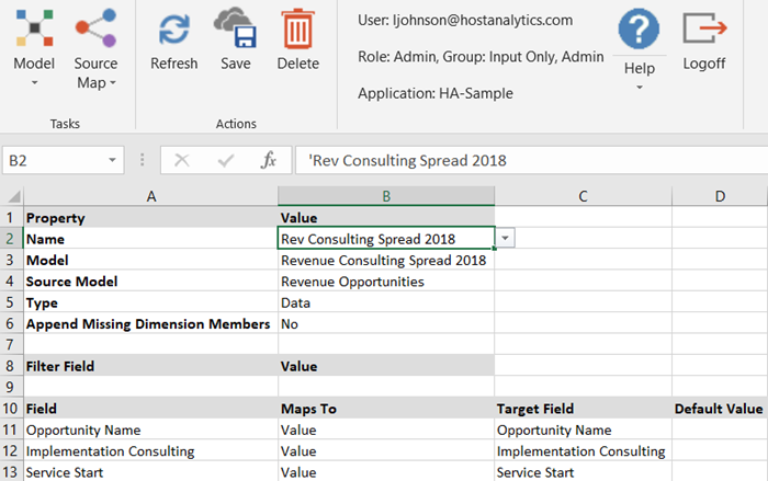
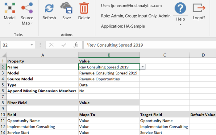
Here is the calculation to run the two ESM maps.

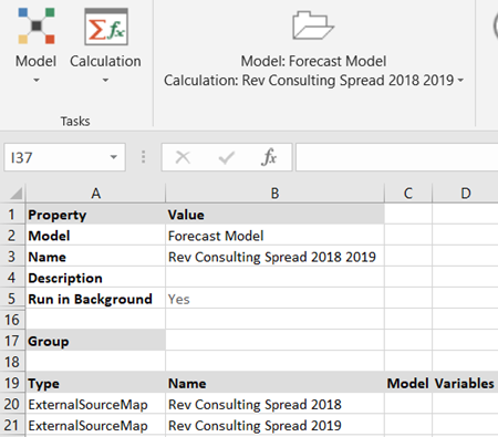
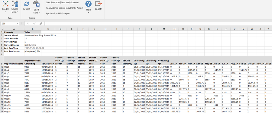
The resulting Consulting Revenue spread data is as follows.

Using Aggregate Functions in Maps

The Aggregate functions are now available in the ESM Maps. You can use these functions directly while moving the data from one ESM to another ESM through maps. The Aggregate Function column has been added to the Maps.

The following Aggregate functions have been included in the maps:

• COUNT

• SUM

• MIN

• MAX

• AVG (average)

The following table provides a quick overview of the functions.

The Aggregate functions were not available in the Maps.

You can use the Aggregate functions, when you have a model with a lot of data and want to compile and organize the raw data into a more consumable and summarized format.

Business Example

If you have a model containing data about Sales opportunities. The model can contain raw data about leads, different sales owners, sales segments, annual recurring revenue (ARR), and so on.

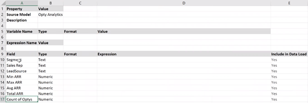
Suppose you want to aggregate data and find specific data related to a sales segment or sales owners. In that case, you can use the aggregate functions available in the map and pull only relevant data to another ESM. The functions provide the flexibility to organize data and identify different key values such as maximum value, minimum value, total count, average, etc.You can create a different model with only relevant fields that are required. The following image shows the model created with only relevant fields.

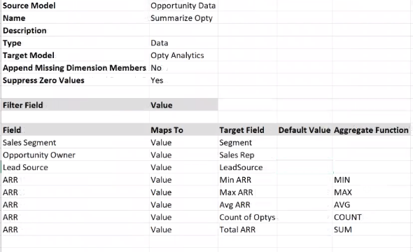
You can create a map with your actual ESM as the Source Model and the new model as the Target model. The following image shows the map containing different fields such as Sales Segment, Opportunity Owner, Lead Source, ARR.

You can group the data as per your requirement and configure the fields accordingly in the Maps. You will have the Aggregate Function column available in the map to select the required function for getting the output. In the example above, the data is grouped by Sales Segment, Opportunity Owner, Lead Source, while the ARR fields are used to find the minimum, maximum, count, average, etc.So, when you run the calculation, you get summarized data that only provides information about the relevant fields.

If you want to filter and segregate data only for a particular field, you can easily do it. For example, you can easily find and track the count, sum, average of opportunities generated by a specific Opportunity Owner.

You can directly find the key point values such as sum, count, maximum, minimum, and average while moving the data from one ESM to another. The functions significantly reduce the effort and time required to organize the data and find key values. You have the flexibility to customize the fields in the map based on your requirement and see different outputs with just a click of a button. You can map a single source field to multiple target fields as per your requirement. For example, ARR was mapped to multiple target fields like sum, count, etc. It is not mandatory to map all the source fields in the map. For example, if you do not want to track data for Lead Source in the example above, then you can just update the Default value for that field to NA and update the Maps to Column value to DimensionFilter. The calculation will aggregate the data based on the updated values and you will see data only based on the Segment and Sales Rep.

In Practice: To use the Aggregate functions in Maps

1. In SpotlightXL, select the Model task and the Map subtask.

2. Select the name of the Source Model defined on the Source Model page.

3. Enter a name for this map.

4. Add the required description.

5. Select the type Data for loading external source data.

6. Select or specify the name of the ESM you want to map the Source ESM to.

7. For Append Missing Dimension Members , select No when mapping to another external source model.

8. Optional, specify the name(s) of one or more fields in the Source ESM to use for filtering the data you want to load. Under the Value column, you can specify a leaf-level field.

9. In the Fields column, specify fields from the Source Model that will be mapped to fields in another External Source Model.

10. Select any of the following in the Maps To column:

    • DimensionFilter : indicates that there is no field in the Source ESM to map to the field in the Target ESM. If you select DimensionFilter, you must specify the Default Value column.

    • Value : indicates that this field in the external source is a value to be copied as is to the specified field in the target ESM.

11. In the Target Field column, select the name of the field in the target ESM to correspond with this field in the source ESM

12. In the Default Value column, specify the text, date, or number that should be placed into this field for all rows in the target ESM if Maps To is DimensionFilter. Or, leave this column blank if Maps To is Value.

13. In the Aggregate Function column, select the required function such as COUNT, MIN, MAX, etc.

Business Use Cases

Let’s understand using the Aggregate functions with some examples.If you have a model containing raw data about leads, different sales owners, sales segments, annual recurring revenue (ARR).

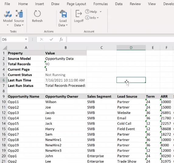
If you want to track your Sales opportunities based on different parameters, for example, you can know the maximum ARR based on Sales Segments, you can know what the opportunities are based on a specific lead source, and many more.

You must perform the following:

• Create a target model with the required fields.

• Create a Map to move data for relevant fields from your Source model to the Target model.

• Select the required Aggregate function.

• Run the calculation to view the output.

Creating a Target Model with Relevant Fields

You must create a Target Model to view and track the data for relevant fields based on your requirement. In this case, as you want to track Sales Opportunities based on different parameters, you can create your Target Model to have fields like Segment, Sales Rep, Lead Source, Minimum ARR, Maximum ARR, and so on.

To do that, navigate to SpotlightXL and create an External Source Model. For example “Opportunity Analytics”

Add the required fields to the Field column of your “Opportunity Analytics” model. If you want to segregate data based on specific fields, then include only those fields to your model. For example, Segment, Sales Rep, Lead Source, Minimum ARR, Maximum ARR, etc.

Once you add fields, specify the type in the Type column. For example, Text, Numeric, Date, and so on. Based on the data in your Source ESM, set the type as Text or Numeric. For example, Segment, Sales Rep, Lead Source are of Type - Text, and the different ARR fields are of Type - Numeric.

In the Include in Data Load column, specify Yes as the value is coming directly from the data source.

Once you have created the Target model and set all the required fields, navigate to creating a Map.

Creating and Configuring a Map

You will be creating a Map to pull the data from your source model to your target model. You must define the Source Fields and then map them to the respective Target Fields. Once you define the source and target fields based on your requirement, you can select the Aggregate functions for the fields. By selecting the Aggregate functions in the Map, you can Aggregate the data as per your requirement while simultaneously moving the data from Source Fields to Target fields. You have the flexibility to configure only the fields that you want to see in the target output.

Let’s understand, configuring a map for different use cases.

Scenario 1

For your Sales Opportunity data, if you want to aggregate data based on Segment, Sales Rep, and Lead Source, and track the Minimum ARR, Maximum ARR, Average ARR, Total ARR, and Count of Opportunities for a Sales Rep in a specific Segment or if you want to know the Lead Source for a Sales Rep’s generated Opportunities.

1. In SpotlightXL, select the Model task and the Map subtask.

2. Select the “Opportunity Data” as the Source Model.

3. Enter a name for this map. For example, “Summarize Opportunity”.

4. Select the type Data for loading external source data.

5. Specify the Target Model name that you created. For example, “Opportunity Analytics”

6. In the Field column, specify the fields that you want to move from your Source Model - Opportunity Data. In this case add Sales Segment, Opportunity Owner, Lead Source, and ARR.

7. Select Value in the Maps To column for the fields that you want to be copied. In this case, specify Value for Sales Segment, Opportunity Owner, Lead Source, and ARR.

8. In the Target Field column, select the name of the fields defined in the target model. In this case, specify Segment, Sales Rep, Lead Source, Min ARR, Max ARR, Avg ARR, Count of Opportunities, Total ARR.

9. Leave the Default Value column blank for all fields.

10. In the Aggregate Function column, select the following for the respective ARR target fields:

    • MIN for the Min ARR field

    • MAX for the Max ARR field

    • AVG for the Avg ARR field

    • COUNT for Count of Opportunities field

    • SUM for Total ARR

The following image shows the Map configuration for the above use case.

Run Calculation with a Map

You must create a calculation for the above Map. The calculation will run the map.

In the Calculation, select the target model name. In this case, select “Opportunity Analytics”.

Select ExternalSourceMap as the type in the Type column.

Specify the name of the map created. In this case, use “Summarize Opportunity”.

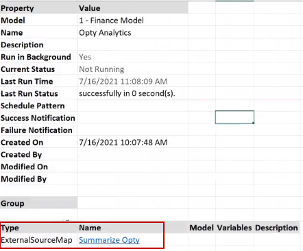
When you run the calculation, you will see that the complete Opportunity data is segregated as per the Map configuration and displayed in the Target Model.

Reviewing Output in the Target Model

Once you run the calculation, you will see that the complete Opportunity data is segregated based on the Sales Segments, Opportunity Owners, Lead Source. Enterprise and SMB. So, based on the fields configured in the Map you would see the data segregated in the output. In this case, as you have mapped the Sales Segment, Opportunity Owner, Lead Source, and ARR source fields with their respective Target fields, you see the values grouped accordingly. You can see the Minimum, Maximum, Average ARR, Total ARR, and Count of Opportunities for all Sales Reps for their Respective Segments. You can also see the Count of Opportunities generated by individual Sales Rep in a specific segment. You can see the lead sources used by a Sale Rep to generate the Opportunity.

Once the data is displayed in columns, you can easily filter data for a specific Sales Rep and track all the details as shown in the above image. For example, if you want to know data for the Sales Rep - Mary, you can just select Mary from the Sales Rep column. Once you select the Sales Rep, you can see the Segments where the Sales Rep has generated the opportunities. In this case, Mary has generated the opportunities in the Enterprise segment, with the total Count of Opportunities generated by her is 8. Out of the total, 7 were generated from the Lead Source “Partner” and 1 was generated from the Lead Source “Partner”. You can also check the Total ARR for Mary along with the other values as Min ARR, MAX ARR, and Average ARR. You can similarly view and track details for any Sales Rep.

Scenario 2

For your Sales Opportunity data, if you want to aggregate data based on Segment, and track the Minimum ARR, Maximum ARR, Average ARR, Total ARR, and Count of Opportunities.

1. In SpotlightXL, select the Model task and the Map subtask.

2. Select the “Opportunity Data” as the Source Model.

3. Enter a name for this map. For example, “Summarize Opportunity”.

4. Select the type Data for loading external source data.

5. Specify the Target Model name that you created. For example, “Opportunity Analytics”

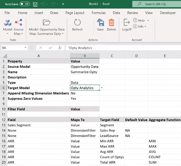
6. In the Field column, specify the fields that you want to move from your Source Model - Opportunity Data. In this case add Sales Segment and ARR. As you previously had Opportunity Owner and Lead Source also there in your Map, now update these fields in the Map and specify “None” in the Field column.

7. Select Value in the Maps To column for the fields that you want to be copied. In this case, specify Value for Sales Segment and ARR, while specify Dimension Filter in the Maps To column for the fields with “None”.

8. In the Target Field column, select the name of the fields defined in the target model. In this case, specify Segment, Min ARR, Max ARR, Avg ARR, Count of Opportunities, Total ARR.

9. In the Default Value column, specify “NA” for the Fields with “None”, and leave this column blank for Sales Segment and ARR fields.

10. In the Aggregate Function column, select the following for the respective ARR target fields:

    • MIN for the Min ARR field

    • MAX for the Max ARR field

    • AVG for the Avg ARR field

    • COUNT for Count of Opportunities field

    • SUM for Total ARR

The following image shows the Map configuration for the above use case.

Run Calculation with a Map

You must create and run the calculation for the above Map configuration. For information on how to create and run a calculation, see Run Calculation with a Map.

Reviewing Output in the Target Model

When you run the calculation for the above configuration, you will see that the complete data is segregated based on the segments Enterprise and SMB.

The Segment column only shows values whereas the Sales Rep and Lead Source columns don’t show any value as they were set to “NA”.

So, based on the fields configured in the Map you would see the data segregated in the output. In this case, as you have only mapped the Sales Segment source field with the Segment target field, you see the values grouped by Segment.

You can see the Minimum, Maximum, Average ARR, Total ARR, and Count of Opportunities for the Enterprise and SMB segment.

The aggregate functions help to compile and summarize huge data from a source system into a consumable output that can easily be used for accurate analysis and tracking.