March 2019 Release Notes

Modeling 2.8.1: Microsoft Office 2019 Support for Modeling

We now support Microsoft Office 2019 in SpotlightXL and Spotlight for Office. See System Requirements.

Modeling 2.8.1: No New Add-In

The SpotlightXL and Spotlight Office Add-Ins were not changed in this release. This release does not require existing users to upgrade their client software.

Modeling 2.8.1: New Look for the Spotlight Login Pages

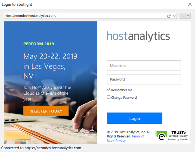
In this release, the look for the login page in SpotlightXL, Spotlight for Office, and Spotlight (Web) is changed.

When you click to login from SpotlightXL, SpotlightWord, SpotlightPPT, or Spotlight (Web), you see the new look. It is similar to the login page for Host Analytics Planning, Consolidation, and Reporting applications. Enter your username and password, then click Login.

Note that there is no change to the URL, username, or password. Only the look and feel of the login page has changed.

Modeling 2.8.1: Converting a Master Model into a Direct Access to PCR Model

In this release, administrators can now convert an existing Master model into a Direct Access to PCR model using Backup and Restore. If the existing Master model was set up with the traditional integration method of connecting to the financial reporting area of PCR, it is possible to switch it over to the newer Direct Access integration method, which has less maintenance. This is accomplished by backing up the Master model with no data and then Restoring it as a Direct Access model.

This functionality is available for all customers.

The traditional method of integration is described here: Modeling: Integration Admin Guide.

The Direct Access method of integration is described here: Modeling: Using Direct Access to PCR Financial Reporting.

Contents

Advantages and Disadvantages of Converting

Pre-Requisites to Converting to a Direct Access to PCR Model

Basic Method to Convert a Master Model to a Direct Access to PCR Model

Detailed Steps to Convert a Master Model to a Direct Access to PCR Model

Details for Administrators

Advantages and Disadvantages of Converting

Using Direct Access to PCR has several benefits:

• No need to manage the data and metadata synchronization between PCR and Modeling. It happens automatically.

• No need to run calculations to move data and metadata.

• Instant access to PCR data and metadata in Modeling.

• The data and metadata reside and are maintained in only one place within PCR.

Using Direct Access to PCR also has some limitations:

• You cannot write back data from within Modeling.

• Views and reports cannot use Save Data or Breakback options.

Pre-Requisites to Converting to a Direct Access to PCR Model

Before a Master model can be converted to a Direct Access to PCR (DAP) model, it must meet the following criteria:

1. All of the data and metadata in the Master model must have been sourced from PCR. In the map that created the Master model, the Source model must be HACPM_Financial.

2. The Master model should have been designed for reporting purposes only (no saving data and no write back to PCR). If there are any views or reports for the Master model, if they had Enable Save, this functionality will not work once the model is converted to a DAP model. It is recommended to turn off Enable Save on views and reports before the conversion.

3. In the map that was used to create the Master model, lookups cannot be used.

4. All the dimensions in the Master model should be sourced from HACPM_Financial. The Master model cannot have dimensions that are not found in HACPM_Financial (the map must not contain target dimension filters).

5. Dimension names must match those in HACPM_Financial.

6. The Master model cannot have a BudgetEntity dimension.

7. The Master model should not have dimensions mapped to HACPM_Financial attributes. While we support the notion of creating attributes as dimensions when sourcing the data from PCR, if the Master model uses this type of mapping, then it cannot be converted into a Direct Access to PCR model.

Basic Method to Convert a Master Model to a Direct Access to PCR Model

The basic method to convert a Master model into a Direct Access model is as follows. Always test the process first in a sandbox or staging environment.

1. Login to Spotlight (web).

2. Backup the existing Master model, with no data.

3. Delete or rename the existing Master model.

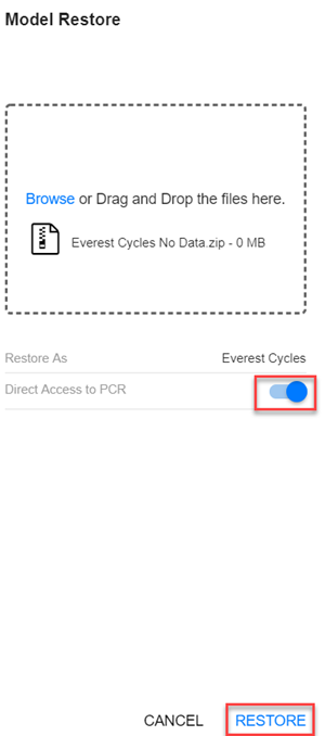
4. Use Restore As to restore the model with the original name and set the flag for Direct Access to PCR.

Detailed Steps to Convert a Master Model to a Direct Access to PCR Model

1. Refresh the application into ModelSBX (customer sandbox) or ModelSTG (staging).

2. Select the Master model to convert to a DAP model.

3. If the Master model has a map with type Metadata or Both, save this map again to validate it. Sometimes, such maps reference deleted dimension members and clicking Save will point out the problems.

4. Verify that the Master model can be converted into a DAP model. See the Pre-Requisites above.

5. Backup the Master model with no data. This creates a local ZIP file.

   Note:

   It is not a bad idea to backup the Master model with leaf-level data as well, so you have an archive of your previous implementation.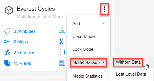

   

6. Clear and delete the original Master model.

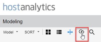
7. Using Model Manager on the Web, click to Restore a model, locate the ZIP file, and check the box to Restore as a DAP model. Ensure the Restore As name has the same name as the original Master model; otherwise, Excel Reports will not work.

   

   

8. Run the calculation on the restored model to refresh the metadata and download alternate hierarchies, attributes, and attribute hierarchies. After this step, the model will be generated and locked.

   

9. Validate views, reports, and Excel Reports for the restored model.

10. Repeat steps 2 through 9 for other models.

If the restored models pass validation, repeat this process in your production environment.

Details for Administrators

• When you Restore a Master model as a DAP model, only one map is retained: the one of type Metadata or Both. All other maps are deleted. The map with type Metadata or Both will be converted into a map with type Metadata. If there is no existing map with type Metadata or Both, a new map with type Metadata will be created by default; it will specify to download All Members for all dimensions.

• When you Restore a Master model as a DAP model, all scopes, formulas, and calculations previously associated with the Master model are deleted. One calculation is created; it is the standard one created with all DAP models, containing five steps to refresh the model. See Hierarchy Updates.

• All existing attributes from the Master model will be deleted. Attributes and attribute hierarchies mapped to the financial cube in PCR will be downloaded. Attributes mapped to a dimension are not supported because, in this case, the Master model would then have a dimension not found in HACPM_Financial. The Master model should not have dimensions mapped to HACPM_Financial attributes.

Modeling 2.8.1: External Source Models Enhanced to Support Transferring Data from One External Source Model to Another External Source Model

In this release, we are adding support for copying data from one External Source Model to another External Source Model. Just as you can copy data from an External Source Model into a Master or Analytic model using an ESM map, now you can use the same method to copy data from one ESM to another. You must first define both the Source and the Target ESMs using the Source Model page, then you can define the Source Map to transfer the data. When the map is run, all data in the Target ESM is deleted before the data transfer from the Source Model is done.

A common use case for this feature would be to store your data load inputs in one ESM and your calculated/formula fields in a second ESM. The formula fields in the second ESM depend on data from the first ESM, so you can copy the requisite fields to the second ESM, which automatically calculates the formula fields. After verifying the data load, then load the data from the second ESM into your Master model.

Contents

Example Source ESM

Example Target ESM

Defining a Map from a Source ESM to a Target ESM

Using a Calculation to Load Data into the Target ESM

Using Filter Fields to Limit the Data Load

Multi-ESM Use Case

Example Source ESM

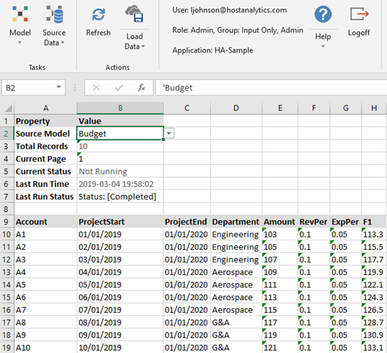
In the examples in this section, the Source Model is Budget. The Source Model has 8 fields.

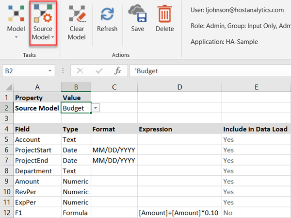
Here is the data in the Source Model.

Example Target ESM

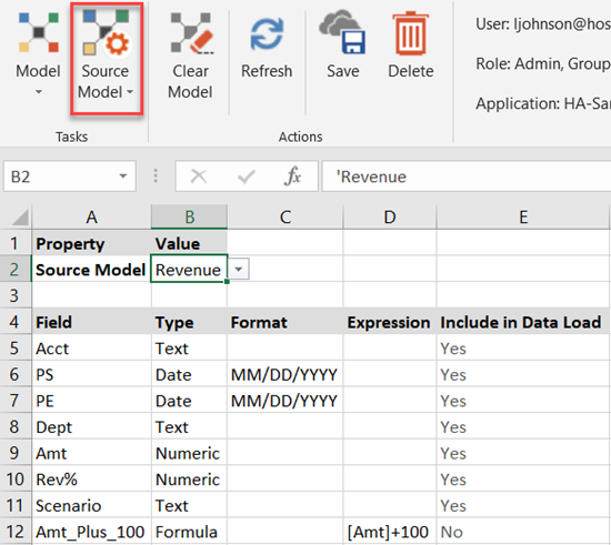
In the examples in this section, the Target ESM is Revenue. The Target ESM also has 8 fields but some fields are different than the Source Model.

Defining a Map from a Source ESM to a Target ESM

The Source Model is a two-dimensional table of data organized into fields. The Target ESM must contain at least as many data-input fields as the Source Model. You will map the fields from the Source Model to the fields in the Target ESM. You must provide a mapping for all the data-input fields in the Target ESM; data-input fields are those marked as Yes for Include in Data Load.

1. Go to Model > External Source Model > Source Map.

2. Enter a name for the map.

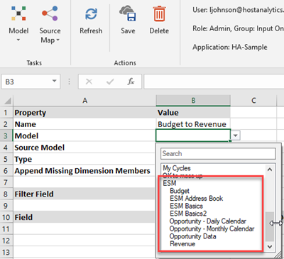
3. From the Model drop-down list box, select or specify the name of the Target ESM you want to map the Source ESM to. In the drop-down list box, the ESMs are listed separately under a sub-heading called ESM.

   

4. Select the Source Model from the Source Model drop-down.

5. Select Data for Type.

6. Set Append Missing Dimension Members to No. This option applies only to mapping to Master or analytic models.

7. Now specify the fields from the Source Model that map to fields in the target ESM. Not all fields in the Source must be mapped, but you must provide a mapping for all the fields in the Target ESM that are marked as Yes for Include in Data Load.

8. For fields in the Target ESM but not in the Source Model, specify Field: None, Maps To: DimensionFilter, the field name in the Target ESM under Target Field, and the text, number, or date to be placed into the target model under Default Value.

   

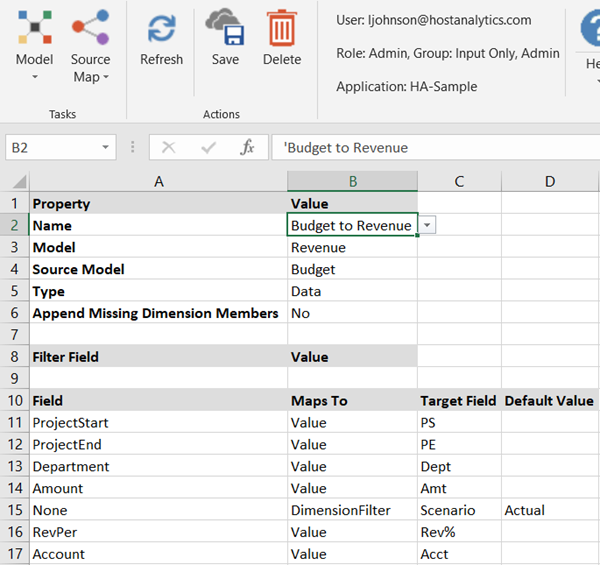
9. Save the map.

Using a Calculation to Load Data into the Target ESM

To copy data from the Source Model to the Target ESM, you must use a calculation to run the External Source Map. When the map is run, all data in the Target ESM is deleted before the data transfer from the Source Model is done.

Calculations are stored within a Master or analytic model. We suggest that you create the calculation inside the Master model that the ESM data will eventually be loaded into.

1. Go to Model > Calculation.

2. Select the Master model associated with your ESMs from the Model drop-down.

3. Give the calculation a name.

4. Create the first step of the calculation by selecting ExternalSourceMap from the Type drop-down.

5. Select the name of the map you created in the previous task from the name drop-down.

6. Save the calculation.

7. Run the calculation.

   

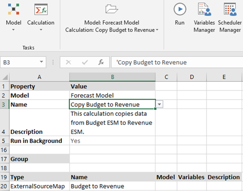
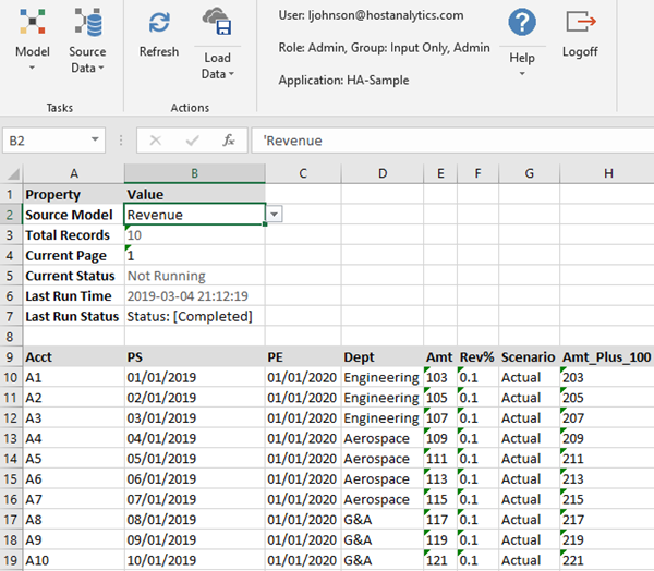
When using this calculation to execute the ExternalSourceMap, the existing records in the Target ESM are deleted, and then records from the Source Model are copied to the Target ESM. To verify the data in the Target ESM:

1. Go to Model > External Source Model > Source Data.

2. Select the Target ESM from the drop-down and click Refresh.

If there were any formula fields in the Target ESM, they are calculated and displayed on the screen.

Using Filter Fields to Limit the Data Load

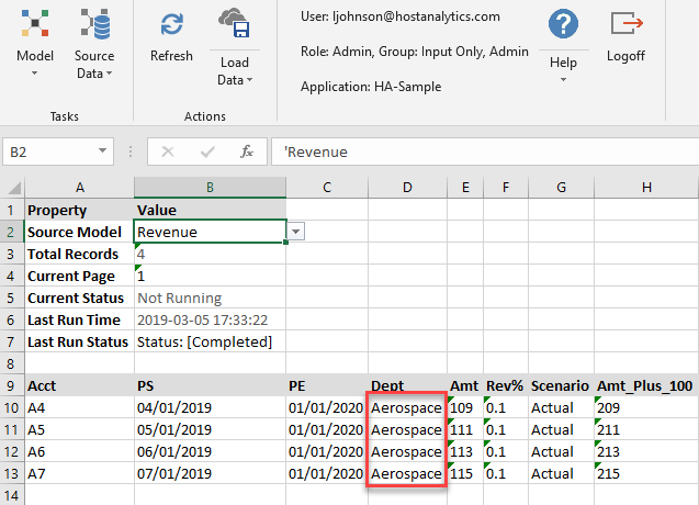
If you want to load only a subset of data in the Source model, use the Filter Field section of the Source Map to indicate which rows of data to load. In the following example, the map indicates that only rows with Department Aerospace should be loaded from Budget to Revenue.

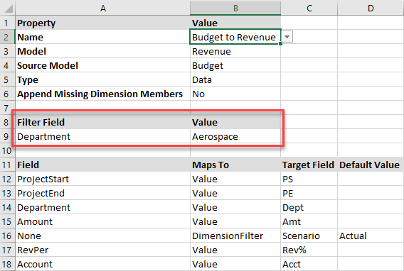
Here is the resulting data.

Multi-ESM Use Case

The following example shows how you can use multiple external source models to generate valuable forecasting data for sales and consulting revenue.

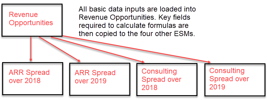
• Data inputs about the prospective customer, sales rep, potential revenue amount (ARR), and potential implementation consulting revenue are loaded into an ESM called Revenue Opportunities.

• Sales revenue is forecast monthly based on a project start date and a term. To keep the ESMs organized and of a manageable size, there is one ESM for each year to store the monthly forecast.

• Consulting revenue is forecast quarterly based on a project start date and four quarters of payments. To keep the ESMs organized and of a manageable size, there is one ESM for each year to store the consulting forecast.

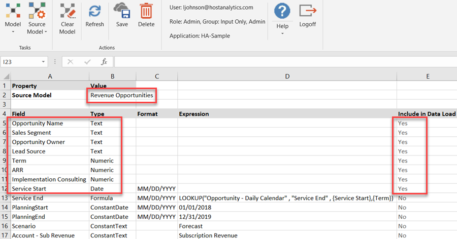
Revenue Opportunities identifies 8 data input fields that you need to load.

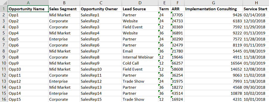
Here is the data load file for Revenue Opportunities.

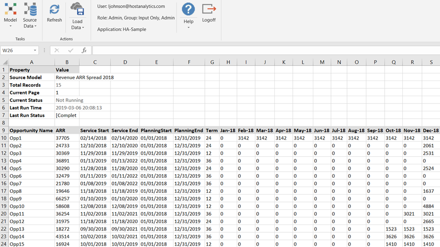
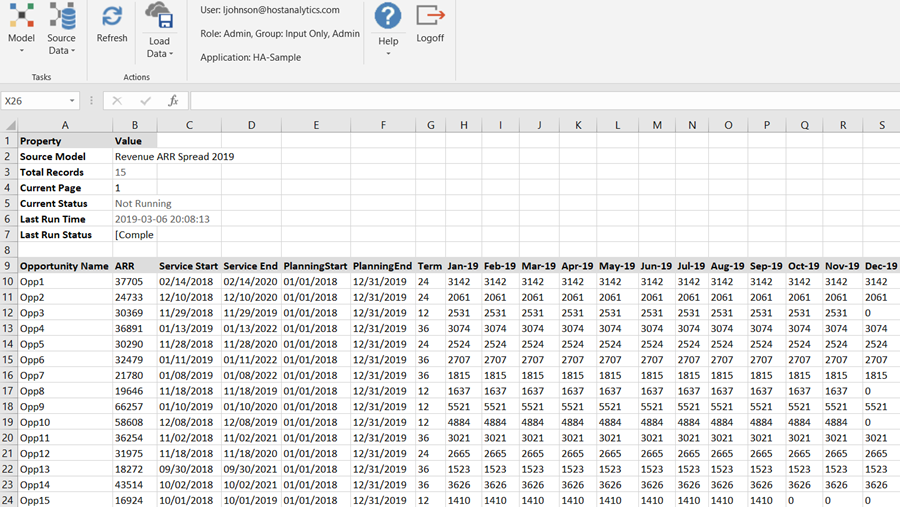
The Revenue ARR amount is spread over 2018 and 2019 in this example. An ESM for each year is created. Only 4 fields from Revenue Opportunities need to be mapped to the ARR Spread models to generate the monthly forecast.

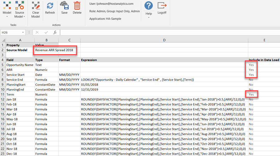
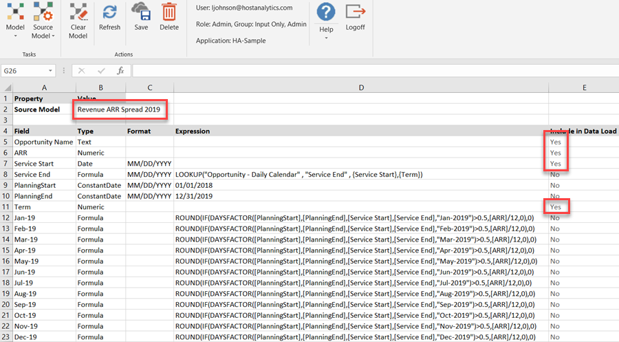
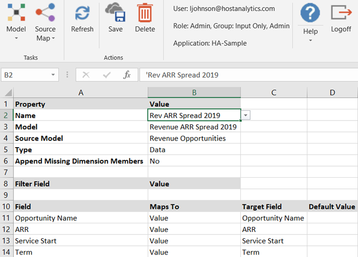
Here are the maps to copy the four input fields from Revenue Opportunities to the Spread models.

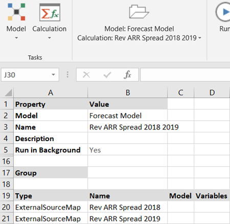
Here is the calculation to run the two ESM maps.

The resulting ARR spread data is as follows. For details on how the DaysFactor function works, see Explanation of the DaysFactor Function.

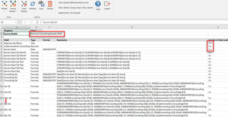
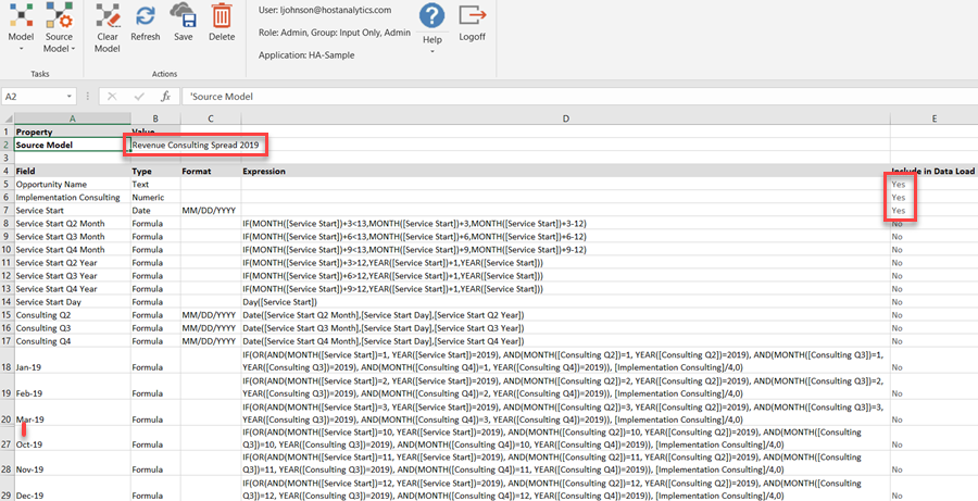
Similar to ARR, the Revenue Implementation Consulting amount is spread over 2018 and 2019 in the following example. To show a different use case, we assume that consulting will be paid in 4 equal quarterly payments and will last no longer than 4 quarters, even if the Term of the project is more than 12 months. An ESM for each year is created. Only 3 fields from Revenue Opportunities need to be mapped to the Consulting Spread models to generate the monthly forecast.

Explanation of the Quarterly Formulas

For syntax of the ESM functions, see External Source Model Field Types, Expressions, and Formulas.

• We have a Service Start date and need to calculate the dates of the following three quarters.

• Formulas are created which calculate what the month and year is 3 months later, 6 months later, and 9 months later.

  • If the Service Start date is late in the year, then adding 3, 6, or 9 months will push into the next calendar year. For example, 11/1/18 plus 3 months is 2/1/19.

  • If you add 3 to the Service Start date month (11 + 3 = 14), and the result is greater than 12, then you need to subtract 12 to get the correct month (14 - 12 = 2).

  • IF(MONTH([Service Start])+3<13, MONTH([Service Start])+3, MONTH([Service Start])+3-12)

  • Similarly with the year, if you add 3 to the Service Start date month (11 + 3 = 14), and the result is greater than 12, then you are into the next year, so you need to add 1 to get the correct year (2018 + 1 = 2019).

  • IF(MONTH([Service Start])+3>12, YEAR([Service Start])+1, YEAR([Service Start]))

• Once you have fields defined that store the month and year of the following three quarters, you can put it all together and create fields to store the Consulting Q2, Q3, and Q4 dates.

  • Date([Service Start Q2 Month],[Service Start Day],[Service Start Q2 Year])

• To create the monthly forecast of consulting revenue, we want 25% of the Implementation Consulting numeric value to appear in each of the four months of the Consulting Q2, Q3, and Q4 dates.

  • For Nov-2018, if the Service Start date, Consulting Q2 date, Consulting Q3 date, or Consulting Q4 date has a Month=11 and a Year=2018, then calculate Implementation Consulting]/4, otherwise 0.

  • In other words, if any of the following conditions are True, then the OR condition is True and will result in [Implementation Consulting]/4.

    • AND(MONTH([Service Start])=11, YEAR([Service Start])=2018)

    • AND(MONTH([Consulting Q2])=11, YEAR([Consulting Q2])=2018)

    • AND(MONTH([Consulting Q3])=11, YEAR([Consulting Q3])=2018)

    • AND(MONTH([Consulting Q4])=11, YEAR([Consulting Q4])=2018)

  • IF(OR(AND(MONTH([Service Start])=11, YEAR([Service Start])=2018), AND(MONTH([Consulting Q2])=11, YEAR([Consulting Q2])=2018), AND(MONTH([Consulting Q3])=11, YEAR([Consulting Q3])=2018), AND(MONTH([Consulting Q4])=11, YEAR([Consulting Q4])=2018)), [Implementation Consulting]/4,0)

 Here are the maps to copy the three input fields from Revenue Opportunities to the Spread models.

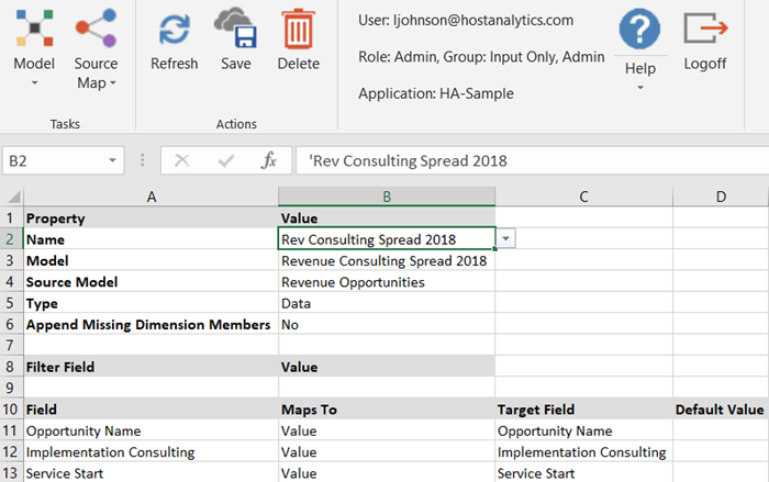
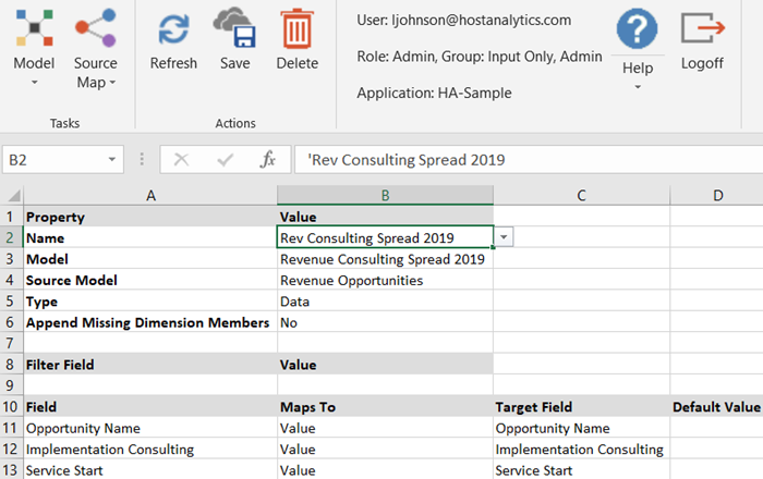
Here is the calculation to run the two ESM maps.

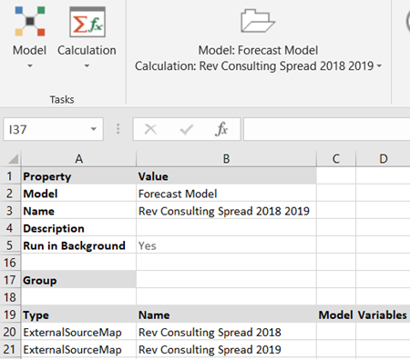
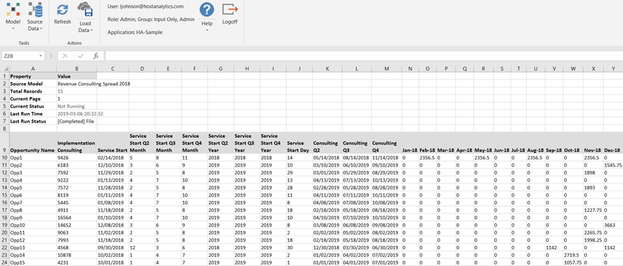
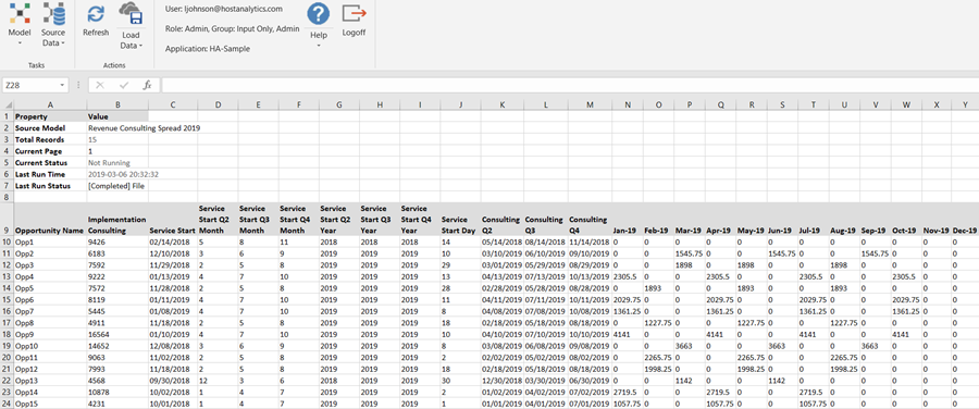
The resulting Consulting Revenue spread data is as follows.

Reporting

Additional Standard Reports Now Available in the Planning Control Panel

The following reports are now available under the Reports tab in the Planning Control Panel:

• Budgeted Data

• Capital Budget Analysis

• Subline Data

Budget Entity and Scenario are updated for the report based on the selections made in the Planning Control Panel.

Platform

Office 2019 Support for PCR

We now support Office 2019. Please see the New Browser Support Matrix.

New Browser Support Matrix

The following browsers and browser versions are supported as of this release:

Data Integration / Other

Enhancement to Scenario Selection in Detailed HR–Employee Data Load Rule (DLR)

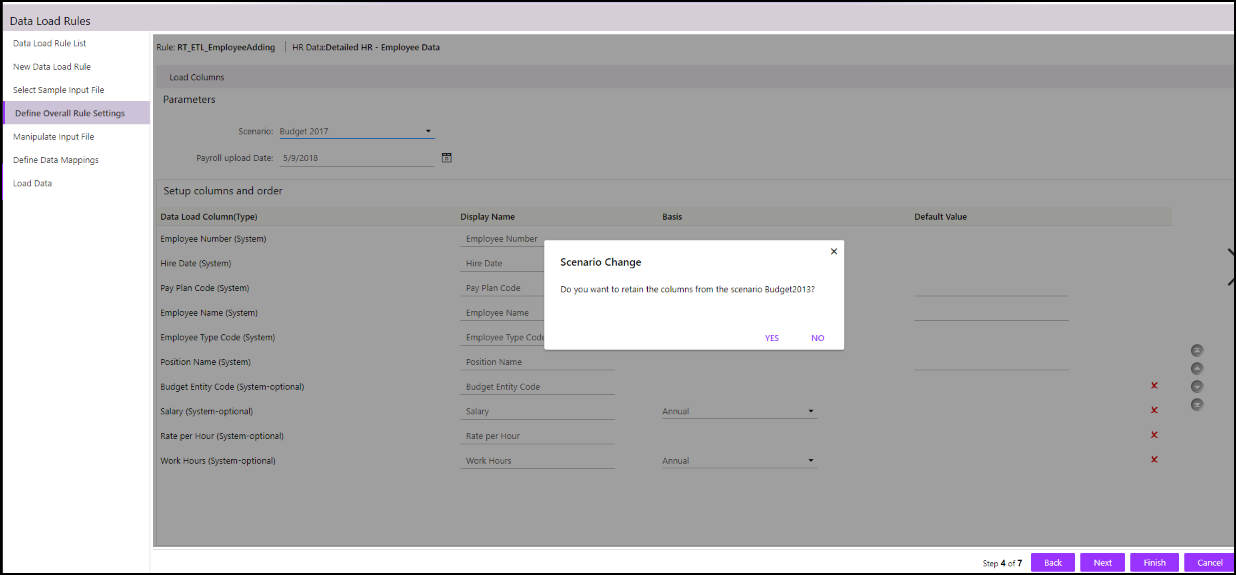
You now have the ability to retain the Data Load Columns when you change the Scenario in the Define Overall Rule Settings tab for a Detailed HR – Employee Data DLR.

For example, when you select Scenario 2 after selecting Scenario 1 from the Scenario drop-down list, the Scenario Change pop-up window displays a confirmation message to retain the columns, and if you click:

• Yes: The columns from Scenario 1 will be retained for Scenario 2.

• No: The columns from Scenario 1 will not be retained for Scenario 2. If there are any columns saved against the DLR for Scenario 2 then those columns will be displayed along with the default columns.

To save the column settings for a scenario, click Next.

The image below displays the Scenario Change pop-up window when you select Budget 2017 scenario after selecting Budget 2013 scenario.

Prior to this release, when you changed the Scenario, the Data Load Columns were not retained. If you wanted to retain the columns, you had to load individual columns and save the settings again.

Common

Update to Application Searchable Drop-downs

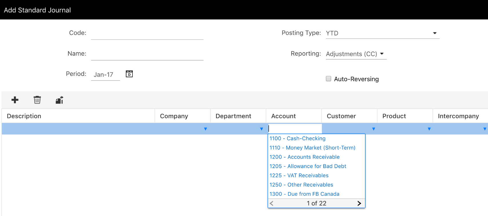
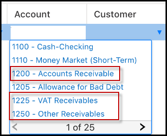
Searchable drop-downs (like the one shown in the image below) are on many application pages throughout the Host Analytics application. Some examples include the Template Setup application page in Planning where you can map segments and the Journals page in Consolidation where you can select segments.

Prior to this release, when you searched within the drop-down, the application would return results based on “begins with” criteria. With this release, when you enter search data in these drop-downs, the application returns results based on “contains” criteria.

In Practice:

Let’s say you know an account “contains” the number 10. You enter 10 in the Account field and (based on the image below) accounts 1100 - Cash Checking and 1110 - Money Market are returned. These accounts are returned because they both “contain” the number 10. Prior to this release, the system would search for an account that “began with” the number 10.

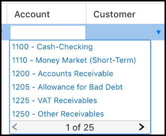
Now, let’s say you search on the word Receivable. There are 3 accounts that contain the word Receivable. So, those accounts shown in the image below will be returned.

Retirement of the Excel Query Add-In

The Excel Query Add-In has been retired. For more information, access the Support Portal and click the following link: https://hostanalyticsinc.zendesk.com/hc/en-us/articles/360015116111-Feature-Deprecation-Excel-Query-Add-In